
In general, any organised data is called a table. But in excel they are not. You need to format your data as a table on excel to get the benefits of tabled data. We will explore those beneficial features of Tables in Excel in this article.
Well, it's easy to create a table in excel. Just select your data and press CTRL+T. Or
And It is done. You have an Excel Table now.
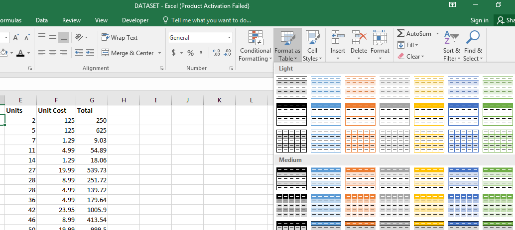
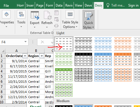
The first visible advantage of an excel table is striped formatting of data. This makes it easy to navigate through rows.

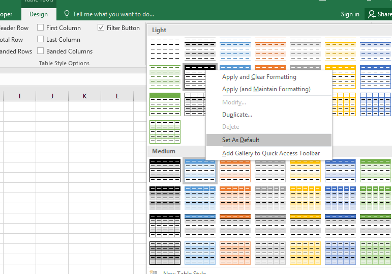
You can select from pre-installed designs for your dataset. You can also set your favourite design as default. Or create a custom new design for your tables.
The pivot tables created with Excel Tables are dynamic. Whenever you add rows or columns to the table, the pivot table will expand its range automatically. It goes for the deletion of rows and columns too. It makes your pivot table more reliable and dynamic. You should learn how to make dynamic pivot tables anyway.
Yes, once you create your charts from an Excel Table, it is dynamic by itself. You don’t need to edit the chart after editing data in a table in excel. The range of chart will extend and shrink as the data in table extends or shrinks.
Each column of tables is converted into a named range. The heading name is the name of that range.
You can easily rename the table.
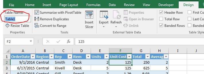
You can’t have two tables with the same names. This helps us in distinction among tables.
I named my table “Table1”, we will use this further in this article. So yeah guys keep following it.
So when you don’t use tables, to count “Central” in the region you would write it like, =COUNTIF(B2:B100,”Central”). You need to be specific about the range. It's not readable to any other person. It will not expand when your data expands.
But not with Excel Tables. The same can be done with excel tables with more readable formulas. You can write:
=COUNTIF(table1[region],”Central”)
Now, this is very readable. Anyone can tell without looking at the data that we are counting Central in the region column of Table1.
This is dynamic too. You can add rows and columns to the table, this formula will return the correct answer always. You don’t need to change anything in the formula.
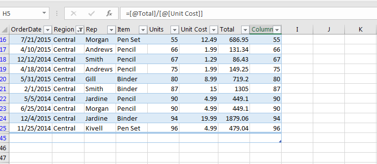
If you write a formula adjacent to the excel table, excel will make that column part of the table and will autofill that column with relative formulas. You don’t need to copy-paste it in the below cells.
One common problem with the normal set of data is that the column headers vanish when you scroll down for data. Only column alphabets can be seen. You need to freeze the rows to make headers always visible. But not with Excel Tables.
When you scroll down, the headers of the table replace column alphabets. You can always see the headers on the top of the sheet.
If you are using multiple sheets with thousands of multiple tables and forget where a particular table is. Finding that table will be hard-won.
Well, you can find a particular table easily in a workbook by writing its name on the name bar. Easy, isn’t it?
Excel Tables have the totals row by default to the bottom of the table. You can choose from a set of calculations to do on a column from SUBTOTAL function, like SUM, COUNT, AVERAGE, etc.
If the total row is not visible then press CTRL+SHIFT+T.
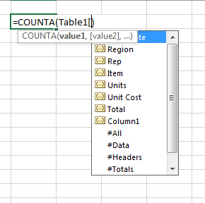
Yup! Like a database, the excel table is well structured. Every segment is named in a structured way. If the table is named as Table1 then you can select all data in a formula by writing =COUNTA(Table1).
If you want to select everything including headers and totals =COUNTA(Table1[#All])
To select the only headers, write Table1[#Headers].
To select only totals, write Table1[#Totals].
To select only data, write Table1[#Data].
Similarly, all columns are structured. To select column fields, write Table1[columnName]. The list of available fields is displayed when you type “tablename[“ of the respective table.
The slicers in excel can’t be used with normal data arrangement. They can be used with pivot tables and excel tables only. In fact, pivot tables are tables in itself. So yeah, you can add slicers to filter your table. Slicers give your data an elegant look. You can see all available options right in front of you. This is not the case with normal filters. You need to click on the drop-down to see the option.
To add a sliver to you table write follow these steps:
The slicers are on now.
Click on items from which you want to apply filters. Like you do on web applications.
Useful, isn’t it?
You can clear all filters by clicking on the cross button on the slicer.
If you want to remove slicer. Select it and hit the delete button.
When you have master data that is stored in the form of a table and you often query the same thing from that master data, you open each time. But this can be avoided. You can get filtered data in another workbook without opening the master file. You can use Excel Queries. This only works with Excel Tables.
If you go to the Data tab, you will see an option, Get External Data. In the menu, you will see an option “From Microsoft Query”. This helps you Dynamically Filter Data from One Workbook to Another in Microsoft Excel.
In a normal data table, when you want to select the whole row containing data, you go to the first cell and then you use CTRL+SHIFT+ Right Arrow Key. If you try SHIFT+Space, it selects the whole row of the sheet, not the data table. But in Excel Table when you press SHIFT+Space, it only selects the row in the table. Your cursor can be anywhere in table row.
One drawback of the table is that it takes too much of memory. If your data is small, it's fantastic to use, but when your data expands to thousands of rows it gets slow. At that time you might want to get rid of the table.
To get rid of the Table, follow these steps:

As soon as you give your confirmation of converting the table to the range, the very design tab will vanish. It will not affect any formulas or dependant pivot tables. Everything will work fine. It's just that you will not have features from the table. And yes, Slicers will go to.
Formating will not go.
Whenever you convert the table to the range, you might expect formatting of the table to be gone. But it won’t. It is suggested to clear the formating first than convert to ranges. Otherwise, you will have to clear it manually.
So yeah guys, this is all I can think about the Excel Tables right now. If you know any other benefits of Tables in Excel then let me know in the comments section below.
Related Articles:
Pivot Table
Dynamic Pivot Table
Sum by Groups in The Excel Table
Use VLOOKUP from Two or More Lookup Tables
Count table rows & columns in Excel
Show hide field header in pivot table
Popular Articles:
How to use the VLOOKUP Function in Excel
The applications/code on this site are distributed as is and without warranties or liability. In no event shall the owner of the copyrights, or the authors of the applications/code be liable for any loss of profit, any problems or any damage resulting from the use or evaluation of the applications/code.


