How to Create Calculated Column(s) in Excel

In this article, we will learn How to Create Calculated Column(s) in Excel.

Scenario

If you want to get the sum of a column by just using the column name, you can do this in 3 easy ways in Excel. Let's explore these ways.

Unlike other articles, let's see with different scenarios first.

How to create a calculated column in a Table:

Select a cell in one of the columns of a Table or a blank cell right to the last column, in the example below the selected cell is G2.
Insert the formula that calculates sales per unit, type the equal (=) symbol, select cell F2, type the divide (/) symbol, and then select cell E2, and press Enter.

The formula is automatically copied to all the cells in the column.

Example :

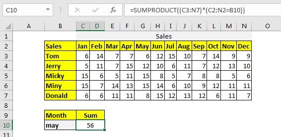
Here I have a table of sales done by different salesmen in different months.

Now the task is to get the sum of given month's sales in Cell C10. If we change the month in B10, the sum should change and return that month's sum, without changing anything in the formula.

Method 1: Sum Whole Column in Table Using SUMPRODUCT function.

The syntax of the SUMPRODUCT method to sum matching column is:

=SUMPRODUCT((columns)*(headers=heading))

Columns: It is the 2-dimensional range of the columns that you want to sum. It should not contain headers. In the table above it is C3:N7.

Headers: It is the header range of columns that you want to sum. In the above data, it is C2:N2.

Heading: It is the heading that you want to match. In the example above, it is in B10.

Without further delay let's use the formula.

=SUMPRODUCT((C3:N7)*(C2:N2=B10))

and this will return:

How does it work?

It is simple. In the formula, the statement C2:N2=B10 returns an array that contains all FALSE values except one that matches B10. Now the formula is

=SUMPRODUCT((C3:N7)*{FALSE,FALSE,FALSE,FALSE,TRUE,FALSE,FALSE,FALSE,FALSE,FALSE,FALSE,FALSE})

Now C3:N7 is multiplied to each value of this array. Every column becomes zero except the column that is multiplied by TRUE. Now the formula becomes:

=SUMPRODUCT({0,0,0,0,6,0,0,0,0,0,0,0;0,0,0,0,12,0,0,0,0,0,0,0;0,0,0,0,15,0,0,0,0,0,0,0;0,0,0,0,15,0,0,0,0,0,0,0;0,0,0,0,8,0,0,0,0,0,0,0})

Now this array is summed up, and we get the sum of the column that matches the column in the cell B10.

Method 2: Sum Whole Column in Table Using INDEX-MATCH function.

The syntax of the method to sum the matching column heading in excel is:

=SUM(INDEX(columns, ,MATCH(heading,headers,0)))

All the variables in this method are the same as the SUMPRODUCT method. Let's just implement it to solve the problem. Write this formula in C10.

=SUM(INDEX(C3:N7,,MATCH(B10,C2:N2,0)))

This returns:

Method 3: Sum Whole Column in Table Using Named Range and INDIRECT function

Everything get's simple if you name your ranges as column headings. In this method, we first need to name the columns as their heading names.

Select the table including the headings and press CTRL+SHIFT+F3. It will open a dialog to create a name from the ranges. Check the top row and hit the OK button.

It will name all the data columns as their headings.

Now the generic formula to sum the matching column will be:

=SUM(INDIRECT(heading))

Heading: It is the name of the column that you want to sum. In this example, it is B10 that contains may as of now.

To implement this generic formula, write this formula in cell C10.

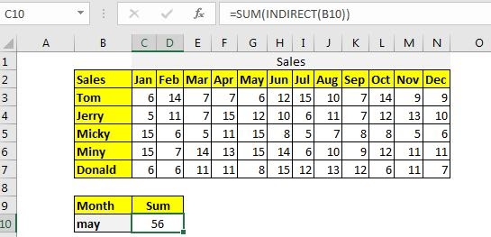
=SUM(INDIRECT(B10))

This returns the sum of May month:

Another method is similar to this. In this method, we use excel tables and it's structured naming. Let's say if you have named the above table as table1. Then this formula will work the same as the above formula.

=SUM(INDIRECT("Table1["&B10&"]"))

Hope this article about How to Create Calculated Column(s) in Excel is explanatory. Find more articles on calculating values and related Excel formulas here. If you liked our blogs, share it with your friends on Facebook. And also you can follow us on Twitter and Facebook. We would love to hear from you, do let us know how we can improve, complement or innovate our work and make it better for you. Write to us at info@exceltip.com.

Related Articles :

How to Sum by Matching Row and Column in Excel : The SUMPRODUCT is the most versatile function when it comes to sum and count values with tricky criteria. The generic function to sum by matching column and row is…

SUMIF with 3D Reference in Excel : The fun fact is that the normal Excel 3D referencing does not work with conditional functions, like SUMIF function. In this article, we will learn how to get 3D referencing working with SUMIF function.

Relative and Absolute Reference in Excel : Referencing in excel is an important topic for every beginner. Even experienced excel users make mistakes in referencing.

Dynamic Worksheet Reference : Give reference sheets dynamically using the INDIRECT function of excel. This is simple...

Expanding References in Excel : The expanding reference expands when copied down or rightwards. We use the $ sign before the column and row number to do so. Here is one example...

All About Absolute Reference : The default reference type in excel is relative but if you want the reference of cells and ranges to be absolute use the $ sign. Here are all the aspects of absolute referencing in Excel.

Popular Articles :

How to use the IF Function in Excel : The IF statement in Excel checks the condition and returns a specific value if the condition is TRUE or returns another specific value if FALSE.

How to use the VLOOKUP Function in Excel : This is one of the most used and popular functions of excel that is used to lookup value from different ranges and sheets.

How to use the SUMIF Function in Excel : This is another dashboard essential function. This helps you sum up values on specific conditions.

How to use the COUNTIF Function in Excel : Count values with conditions using this amazing function. You don't need to filter your data to count specific values. Countif function is essential to prepare your dashboard.