In this article, we will learn How to create SEO tool in Excel.
I thought why not use Excel for SEO. Excel provides a wide range of analytical formulas and tools to conduct analysis. In this article, we will learn how to create a tool in excel and use it for SEO purposes.
| Note: Throughout the article, we will use named ranges. All columns will be named as per their headings. This will make it easy to understand. If you don’t know about named ranges, read it here. |
How to Validate Redirects
While migrating to a new domain, a website reform, an update or any xyz reason, you might redirect your website or web page to a new address. It is very reasonable to check if the website or web pages are redirected properly. In excel, you can do it easily. Just using IF function.
Consider this data fetched from the SEO tool.
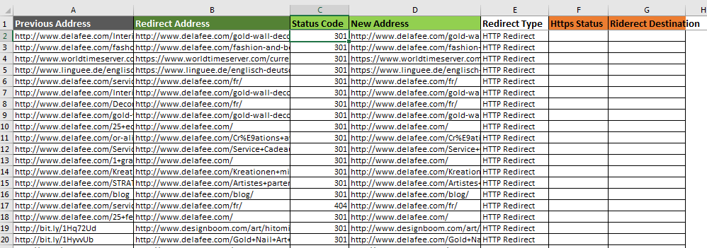
The addresses in column A needed to be redirected to Addresses in column B.
The column A is named as Previous Address and column B as Redirect Address.
In column C, we have status code. 301 is for successful redirection. The column C:C is Named as status code.
In Column F, we will check Http status code. If status code is 301 then we will print Redirected. Else we will show “Error” with status code in C.
Write this IF formula in column C and copy down the cells.
| =IF(Status_Code=301,"Redirected","Error: "&C2) |
In column G, we will check if the page is redirected to the intended URL. For this, Redirect Address and New Address should be the same. We will compare these two columns using Excel IF in column G Redirected to Destination. If the page is being redirected to right page, we will show “Yes” else “No”
| =IF(Redirect_Address=New_Address,"Yes","No") |
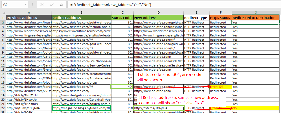
I used conditional formatting to highlight cells having specific text. Now it's easy to see problematic cases.
To highlight errors, select the F column and...
Go to home? Conditional Formatting? Highlight Cells Rules? Text that contains:
Write “Error” in the dialogue box. Hit Ok.

Choose default formatting or a customised formatting.
Do the same for Redirected to Destination (G column). Just write “No” in the text box.
Comparing Clicks, Impression, Average CTR and Average Position of Keywords In Excel, Better than Search Console.
The Google Search Console does provide comparisons over period visually in graph but in numerical data, you have stress up your eyes. You have to see numbers in both time frames to know how much difference is there.
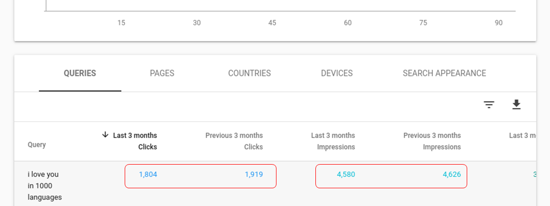
It would be better, if it could show how much better or worse the keyword is doing on our site. We can do this in excel.
To do comparison of keyword on site, over two time period in excel, follow these steps.

(I will reduce the column width of ‘data from search console’ columns, so that it fits on the screen.)
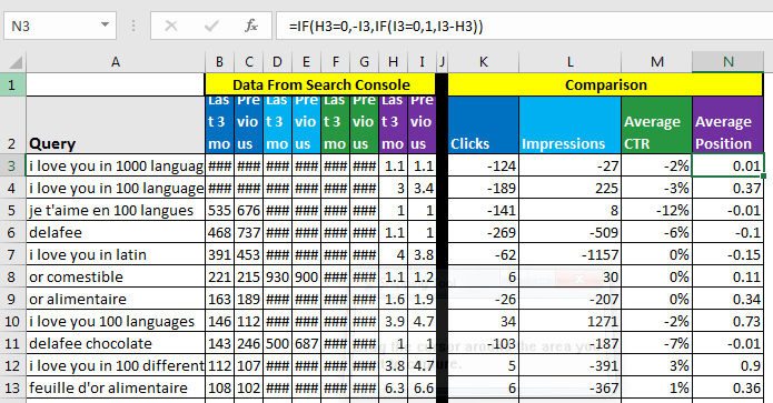
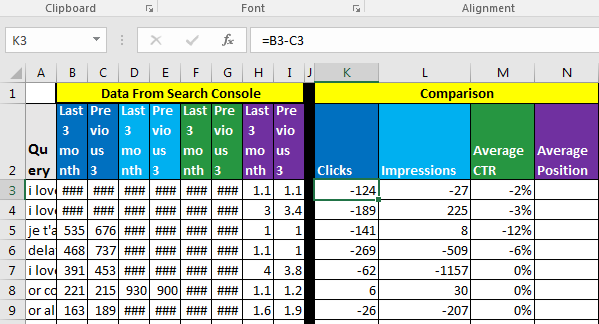
Here, I have just copied data from the search console in Column A to G. In K, L, M and N we will compare the two time periods of Clicks, Impressions, CTR, and Position. I will conditionally format cells green if there is improvement and red text if there is deterioration. If there is no change then no formatting. Just black text with white background.
Write these formulas in K3, L3, and M3 respectively.
| =B3-C3 |
| =D3-E3 |
| =F3-G3 |
We are just subtracting previous months data from last month's data. A positive number indicates improvement, negative deterioration, and 0 indicates no change.
In N3, write this formula. Why?
| =IF(H3=0,-I3,IF(I3=0,1,I3-H3)) |

The average position case is different. Increment in position means your page is ranking low which bad. Decrement in position means your page is moving toward the 1st position. It should not be 0. 0 means your page is not being considered for that keyword.
Here what we need to do,
If Last 3 month’s position is 0, then we have dropped from the previous month's position to 0 which means minus previous month’s position (-I3).
If Previous 3 month’s position is 0, then we have at least ranked, hence we will mark improvement as 1.
And if none of them are 0 then we will simply subtract last month's position from previous month’s position. Positive is good, and negative is bad.

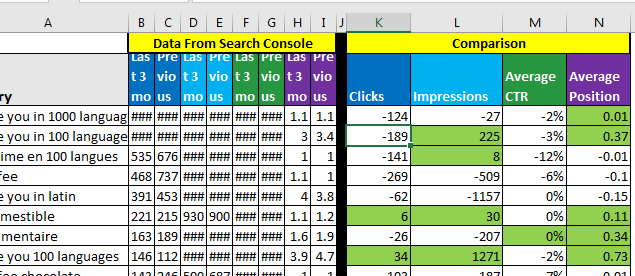
Now you can see all the positive changes in green cells.
Now for negative numbers, we can either use conditional formatting or cell formatting. I am using cell formatting.
Select the columns. Press CTRL+1 to open cell formatting.
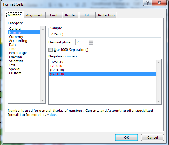
From categories, select numbers. Choose red text witt closed parenthesis.
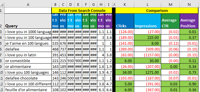
All these red numbers indicate depreciation in clicks, impressions, CTR and position for the respective query.
Merge Search Performance Matrics with Backlinks Data to See Which Page Needs More Backlinks
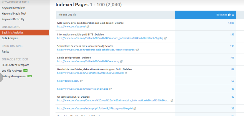
The Search console only provides keyword performance on one page of the site. Google Analytics provides data pages ranking on your site. And backlinks data we get from tools like SEMrush. Using VLOOKUP Function of Excel, you can merge all these tables.
Query and Site Data
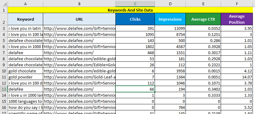
Backlink Data
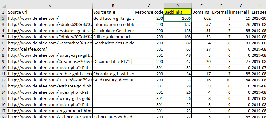
We Need Backlink Data in Query and Site Data sheet.
Write this VLOOKUP formula in Backlink Data Table.
| =IFERROR(VLOOKUP(B3,Backlinks!$A$2:$D$2041,4,0),"No Backlinks") |
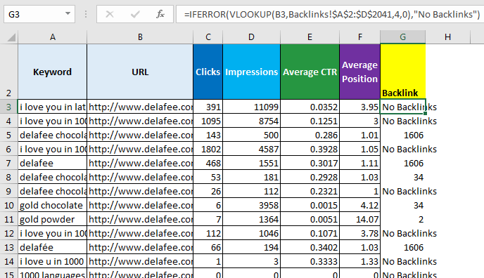
The VLOOKUP function will retrieve all backlink data in one sheet using URL. If URL is not found in the backlink sheet then IFERROR Function will return “No Backlinks”. Now you can know which pages need backlinks to be added to improve performance on certain queries.
Hope this article about How to create SEO tool in Excel is explanatory. Find more articles on calculating values and related Excel formulas here. If you liked our blogs, share it with your friends on Facebook. And also you can follow us on Twitter and Facebook. We would love to hear from you, do let us know how we can improve, complement or innovate our work and make it better for you. Write to us at info@exceltip.com.
Popular Articles :
How to use the IF Function in Excel : The IF statement in Excel checks the condition and returns a specific value if the condition is TRUE or returns another specific value if FALSE.
How to use the VLOOKUP Function in Excel : This is one of the most used and popular functions of excel that is used to lookup value from different ranges and sheets.
How to use the SUMIF Function in Excel : This is another dashboard essential function. This helps you sum up values on specific conditions.
How to use the COUNTIF Function in Excel : Count values with conditions using this amazing function. You don't need to filter your data to count specific values. Countif function is essential to prepare your dashboard.
The applications/code on this site are distributed as is and without warranties or liability. In no event shall the owner of the copyrights, or the authors of the applications/code be liable for any loss of profit, any problems or any damage resulting from the use or evaluation of the applications/code.