Array Formula in Microsoft Excel 2010

To avoid the errors while using the function to combine multiple conditions in Array formulas, we use “AVERAGE”, “IF”, “ISNUMBER”, and “AND” function in Microsoft Excel 2010.

Average:- This function is used for returning the average (arithmetic means) of its arguments that can be numbers or names, arrays or reference that contains numbers.

The syntax of AVERAGE formula:-  =AVERAGE(number1,number2,……)

Let’s take an example to understand how the Average formula performs.

We have a list in the range A2:A11. Now, we want to see the average number in the list.

Follow the below given steps:-

• Select the cell B2, and write the formula in the cell.
• =AVERAGE(A2:A11)
• Press Enter on the keyboard.
• The function will return the 34, which is the average of the range.

ISNUMBER: This function can be used to check if a cell contains a number.

Syntax of “ISTEXT” function:       =ISTEXT (value)

Example: Cell A2 contains the text 123

                        =ISNUMBER (A2) and then function will return “TRUE”

               Cell A3 contains the number “XYZ”

                        =ISNUMBER (A3) and then function will return “FALSE”

IF: - Check whether a condition is met and returns one value if True and another value if False.

The syntax of “IF” function =if(logical test,[value_if_true],[value_if_false])

First the formula will do the logical test, what if the output of logical test is true and false.

For example: Cell A2 and A3 contain the number 3 and 5. If the number is 3, the formula should display “Yes”, else “No”.

=IF (A1=3,"Yes","No") 

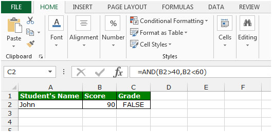
AND:- This function is used to check whether all the arguments are true and returns TRUE if all the arguments are TRUE.

The syntax of “AND” function =AND(logical1,[logical2],….)

For example: Cell A1 contains student name, B1 contains 50, and we need to check the criteria.

• If the cell contains the number more than 40 and less than 60.
• Write the formula in cell C1
• =AND(B2>40,B2<60), press Enter.
• The function will return True.
• If we will change the number less than 40 and greater than 60, the function will return False. 

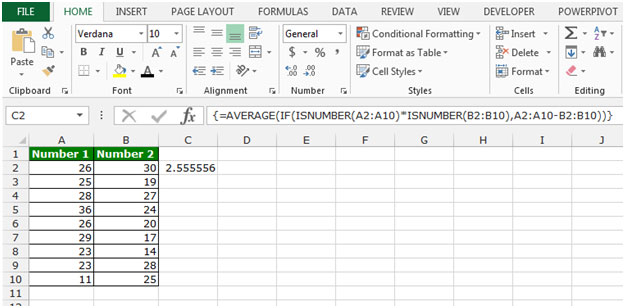
Let’s take an example to understand how we can avoid the errors when using the And function to combine multiple conditions in Array formula.

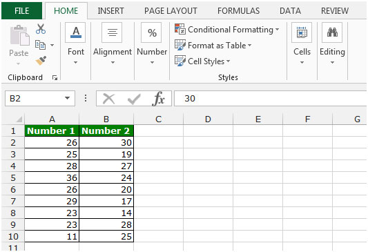
We have data in range A2:B10. Column A contains the list of number 1 and column B contains number 2.

To avoid errors when using the AND function to combine multiple conditions in Array formulas, follow the below given steps:-

• Write the formula in cell C2.
• =AVERAGE(IF(ISNUMBER(A2:A10)*ISNUMBER(B2:B10),A2:A10-B2:B10))
• Press Ctrl+Shift+Enter on your keyboard.
• After pressing the Ctrl+Shift+Enter, function will look like this {=AVERAGE(IF(ISNUMBER(A2:A10)*ISNUMBER(B2:B10),A2:A10-B2:B10))}
• The function will return the average difference between each pair of values in Column A and B.

This is the way we can avoid the errors while using the AND function to combine multiple conditions in Array formulas in Microsoft Excel.