In this article, we will learn how to use conditional formatting to compare two arrays to show difference in excel.
Conditional Formatting in Excel is used to highlight the data on the basis of some criteria. You can use this to compare two lists in excel and visualize data to make worksheets easier to understand.
How to solve the problem?
First we need to understand the logic behind this task. To compare lists we need to match the cell values and keep a record of matched values. On the basis of the record we highlight the cells which differ from the other list.
First we will understand the logic behind it via using the formula on data.
EXAMPLE:
Here we have two lists of Names, One is Guest list and another is an invitation list. We need to highlight the guest who didn't appear and the guest who appeared without invitation.
We will construct a formula to compare two lists. For this we will use COUNTIF function. COUNTIF function returns the count of cells satisfying the given criteria.
Generic formula:
Array1 : list of values in the first column
Value1 : first value from the second column list

These 2 lists look similar but there are differences. To highlight those differences we will use the formula in D2 cell
Write the formula in the D2 cell.
Formula
array1 ( C2:C14 ) referred as named range
array2 ( E2:E14 ) referred as named range
Explanation :
COUNTIF function matches the C2 cell in array2 and returns its occurrence in number.
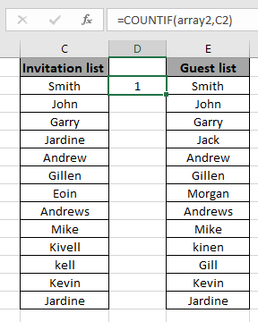
Copy the formula in other cells, select the cells taking the first cell where the formula is already applied, use shortcut key Ctrl + D or using the drag down cell option in excel.
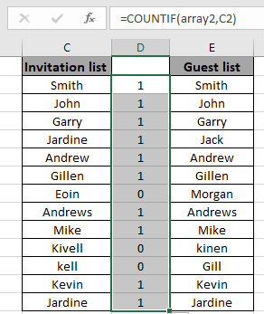
Here is what we needed. These 1s and 0s indicate whether the value is in the array or not.
You can use this formula to highlight list cells. For this, we will use conditional formatting tool of excel.
Now we will apply conditional formatting to the first list. Then we will proceed to the second list
Select the first array or array1.
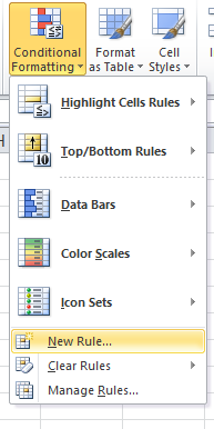
Select Home > Conditional Formatting > New Rule.
A dialog box appears and choose Use a formula to determine which cells to format option. Then a formula box appears.
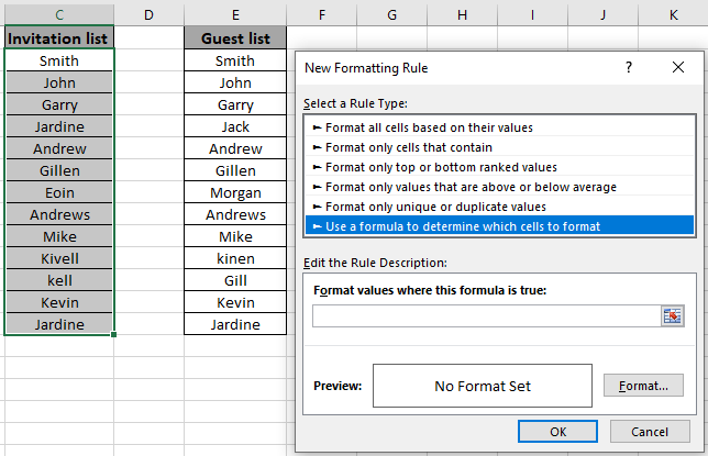
Use the formula in the formula box.
Explanation :
COUNTIF function matches the C2 cell value with array2 and returns its occurrence in number.
=0 : this is used to highlight only the cells which equals the formula to zero.
Fill Format with Green colour and click OK.
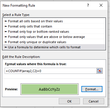
Click Ok to get the names of the guests who were invited but didn't showed up.

As you can see excel change cell color based on value of another cell using Conditional formatting tool.
Now perform the same structure with the second list.
Select the first array or array1.
Select Home > Conditional Formatting > New Rule.

A dialog box appears and choose Use a formula to determine which cells to format option. Then a formula box appears.

Use the formula in the formula box.
Explanation :
COUNTIF function matches the E2 cell value with array1 and returns its occurrence in number.
=0 : this is used to highlight only the cells which equals the formula to zero.
Fill Format with Red colour and click OK.
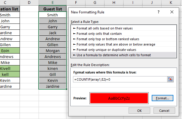
Click Ok to get the names of the guests who weren't invited but anyhow showed up.
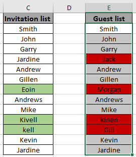
As you can see changed cell color based on value of another cell using Conditional formatting tool.
Hope you learned how to use conditional formatting in Excel used to Compare two list and highlight the differences. Explore more conditional formulas in excel here. You can perform Conditional Formatting in Excel 2016, 2013 and 2010. If you have any unresolved query regarding this article, please do mention below. We will help you.
Related Articles:
How to use the Countif function in excel
Relative and Absolute Reference in Excel
Shortcut To Toggle Between Absolute and Relative References in Excel
All About Named Ranges In Excel
Total number of rows in range in excel
Popular Articles:
The applications/code on this site are distributed as is and without warranties or liability. In no event shall the owner of the copyrights, or the authors of the applications/code be liable for any loss of profit, any problems or any damage resulting from the use or evaluation of the applications/code.