In this article, you will learn how to format row above the matched criteria.
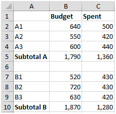
For example:

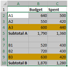
The criterion is to look for text Subtotal in the above table & then color the row which is just above to Subtotal.
We will use a combination of ISNUMBER & SEARCH functions to get the output.
ISNUMBER: Checks whether a value is a number, and returns TRUE or FALSE.
Syntax =ISNUMBER(value)
value: It is the value that you want to check whether it is a number or not.
The SEARCH function returns the number of the character at which a specific character or text string is first found, reading left to right (not case-sensitive)
Syntax =SEARCH(find_text,within_text,start_num)
find_text: The text that you want to find.
within_text: Itis the text in which you want to search.
start_num: This is optional. It is the number in the string from which you want to extract data.
Select the range A2:C10
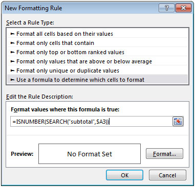
Open the New Rule Manager from Conditional Formatting or press ALT + O + D
Select “Use a formula to determine cells to format”
Enter the formula as =ISNUMBER(SEARCH("subtotal",$A3))

Click on Format to apply color & then click on OK button twice.

In this way, we can easily format the row above the matched criteria.
The applications/code on this site are distributed as is and without warranties or liability. In no event shall the owner of the copyrights, or the authors of the applications/code be liable for any loss of profit, any problems or any damage resulting from the use or evaluation of the applications/code.