Get Relative COLUMN index in excel

In this article, we will learn about how to Get Relative Column index in excel.

For instance, we have data and we need to mark the index for the data having index column. But the problem is that the data doesn't start from the 1st Column of the worksheet. So we will use the Column function and a simple logic to get the column Index in the data. Let's get some understanding for the Column function first.

The Column function returns the Column number of the cell or the cell reference. It returns a number for the given cell reference.

Syntax:

= COLUMN ([cell_reference])

Note: If no argument is given to the function. Then the function returns the Column number for the cell where formula is used.

Now we will construct a formula using the above explained function and a simple logic. Firstly, we need to get the first index which is 1. So we need to create a difference of 1 between 2 numbers. These two numbers
will be the outcome of two Column functions. Then for the rest of the table we just be extending the same formula till the last Column of the data.
Generic formula:

= COLUMN( ) - COLUMN( cell_ref )

Explanation:

COLUMN( ) function returns the Column number for the cell where used.
Now we want difference of 1. So we take cell reference of the left adjacent cell using the COLUMN ( cell_ref ).
The difference will automatically create column index.

Let’s understand this function using it in an example.

Here we have a data_table with names and

We need to mark each column with its index in the given Index Row.
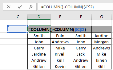
Use the customized formula in the D2 cell:

= COLUMN( ) - COLUMN ( $C$2 )

Explanation:

Column ( ) will return 4, the corresponding Column number for the cell.
Column( $C$2 ) will return 3, the Column number for the Column C.

$ sign returns the relative cell reference which is used to fix the cell reference.

The formula will look like as shown in the snapshot above. Click Enter to get the result.

As you can see in the above snapshot that the formula returns 1 as the first INDEX for the table. Copy the formula to the rest of the cells using the Ctrl + R shortcut key or drag right feature of excel.

As you can see from the above snapshot that the index column is filled with values as required.
There's a new and easy method to the same. In Excel 2016, it automatically extends the values just by the drag down option. Follow the steps to see how it is used.

Type the number 1 & 2 in the first and second Index space.
Then select the two cells and drag it right from the bottom till the column Index fills.

As you can see in the gif above that the INDEX column is done.
Hope you understood how to Get Relative Column index in Excel. Explore more articles on Excel cell reference function here. Please feel free to state your query or feedback for the above article.