In this article, we will learn Highlight Duplicates Except First Number in Range in Microsoft Excel.
Scenario :
Earlier we learned how to highlight the entire if any cell in row contains specific text. Now we will learn how to separate duplicate values where the first occurrence is considered as a unique value. For example: In an array of 1 , 2 , 3 , 1 , 4 & 5 , Only the 1 at 4th number will be coloured differently. Separation is done on the basis of cell format. So we know conditional formatting is our tool.
we will highlight the row using conditional formatting.
Generic Formula in Conditional Formatting
| = COUNTIF ( $R$1:R1 , >1) |
Cell with relative row: this is a cell reference where the column is absolute and row is relative. For example $A$1 (fixed row and column) and $A1 (fixed row) and A$1 (fixed column) . Learn in detail about referencing in excel here.
> 1 : It is the criteria that you want to match and highlight.
Example :
All of these might be confusing to understand. Let's understand how to use the function using an example. Here I have some data on fruits. I just want to highlight the entire row if the fruit rate is greater than 100.
Select the row of table (A2:C2).
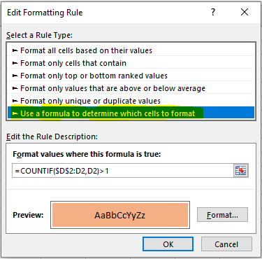
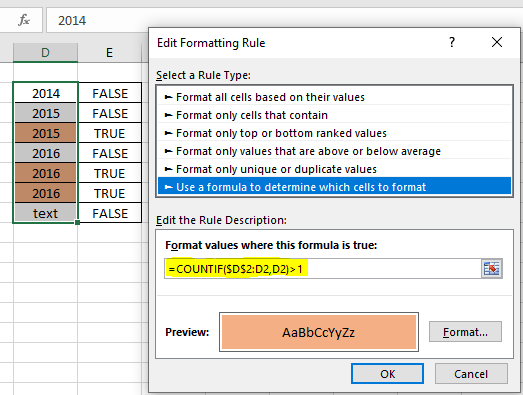
| =COUNTIF($D$2:D2,D2)>1 |
It is necessary to select the entire row before doing conditional formatting.

Copy this range and paste the special format to the entire table.

Now each cell will be highlighted whose frequency or occurance is greater than 1. Here I have hardcoded the criteria, but you can give cell reference too.
How does it work?
Well, it is quite simple. Here the formula just colours the cell where count of value comes greater than 1. In the first occurrence of the value, the count remains 1.
Note that only the cell $D$2 is frozen using $ and row are left relative. It is because we want to change the lookup row when we copy the conditional formatting and the column stands absolute. In the end we get highlighted cells that contain values greater than 1. Learn about referencing in detail here.
So yeah guys, this is how you can highlight the entire row based on cell value or criteria. This is quite easy if you understand absolute and relative referencing in excel.
Here are all the observational notes regarding using the formula.
Notes:
Hope this article about how to Highlight Duplicates Except First Number in Range in Microsoft Excel is explanatory. Find more articles on calculating values and related Excel formulas here. If you liked our blogs, share it with your friends on Facebook. And also you can follow us on Twitter and Facebook. We would love to hear from you, do let us know how we can improve, complement or innovate our work and make it better for you. Write to us at info@exceltip.com.
Related Articles :
Find the partial match number from data in Excel : find the substring matching cell values using the formula in Excel.
How to Highlight cells that contain specific text in Excel : Highlight cells based on the formula to find the specific text value within the cell in Excel.
Conditional formatting based on another cell value in Excel : format cells in Excel based on the condition of another cell using some criteria in Excel.
IF function and Conditional formatting in Excel : How to use IF condition in conditional formatting with formula in Excel.
Perform Conditional Formatting with formula 2016 : Learn all default features of Conditional formatting in Excel.
Conditional Formatting using VBA in Microsoft Excel : Highlight cells in the VBA based on the code in Excel.
Popular Articles :
How to use the IF Function in Excel : The IF statement in Excel checks the condition and returns a specific value if the condition is TRUE or returns another specific value if FALSE.
How to use the VLOOKUP Function in Excel : This is one of the most used and popular functions of excel that is used to lookup value from different ranges and sheets.
How to Use SUMIF Function in Excel : This is another dashboard essential function. This helps you sum up values on specific conditions.
How to use the COUNTIF Function in Excel : Count values with conditions using this amazing function. You don't need to filter your data to count specific values. Countif function is essential to prepare your dashboard.
The applications/code on this site are distributed as is and without warranties or liability. In no event shall the owner of the copyrights, or the authors of the applications/code be liable for any loss of profit, any problems or any damage resulting from the use or evaluation of the applications/code.