Hlookup in Excel 2010

In this article we will learn about Hlookup function in Excel 2010.

HLOOKUP: The function is used to look for a value in the top row of a table or array of values and return the value in the same column from a row you specify.

Syntax of “HLOOKUP” function:            =HLOOKUP(lookup_value,table_array,row_index_num,[range_lookup])

Uses of Hlookup Function

We used this function to pick the values from one data to another, but the condition is we should have the common values in both data’s so we can easily pick the value.

Let’s take an example and understand how and where we can use Hlookup function in Microsoft Excel 2010 and 2013.

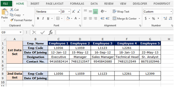
Example 1: We have 2 data sets. In which we have require joining date from 1^st data to 2^nd data.

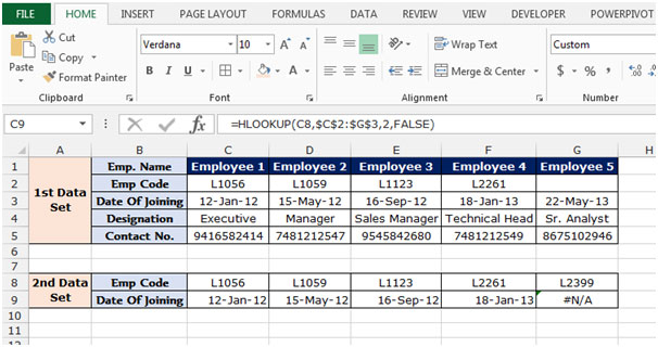
To pick the value from 1^st data to 2^nd data we have common value is Emp. Code, So we will put the Hlookup function through Emp. Code follow below mentioned steps to pick the joining date:-

• Select the cell C9 and write the formula.
• =HLOOKUP(C8,$C$2:$G$3,2,false)  press enter.
• The function will return the joining date for this L1056 Emp code.
• To return the date of joining to all the employees, Copy the same formula and paste in the range D9:G9.

Note: If we do not have the common value in other data from which we want to pick the data, formula will give the #N/A error. As you can see in above snapshot the employee code L1089 in not available in 1^st data set so formula is giving the error.

This is all about the Hlookup function in Microsoft Excel 2010 and 2010.