How to apply Conditional Formatting in a cell before a particular character

How to apply Conditional Formatting in a cell before a particular character

Scenario:

Sometimes given a list of numbers and we need to highlight data numbers on the basis of some criteria. For example: we need to highlight numbers less than or equal to some value. But the problem occurs if the data has approximate results. Given an example we need to highlight how much sales are done which are greater than or equal to 50000, in a data where sales values are marked with symbols like ">60000". So we need a formula for the data which highlights numbers and symbol matching values.

How to solve the problem?

For this we will be using the Conditional formatting obviously and some excel function listed below.

1. IF function
2. ISNUMBER function
3. LEFT function
4. MID function
5. LEN function

The combination of the formula first checks if the value is a number or not. If the number matches criteria, it returns True or False. But if the value is a number with operator, then the formula finds the operator(<) and matches the remaining value (number) with the criteria.Below is the generic formula to match value less than or equal to criteria.

Generic formula:

cell : cell reference to check

criteria : criteria value to match with

< : operator to match criteria

Example :

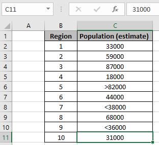
All of these might be confusing to understand. Let's understand this formula by running it on an example. Here we have data with estimated population for each region.

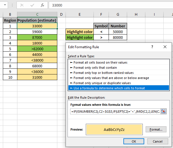
Here as you can see the data have values (numbers with operator) which need to be considered too. We need to highlight cells which have a population less than 50000. So we use the formula stated below with Explanation under Conditional formatting formula box.

Go to Home -> Conditional formatting -> New Rule

A dialog box appears in front select Use a formula to determine which cells to format -> input the below formula under the Format values where this formula is True:

Use the formula for matching value less than 50000.

Explanation:

1. First IF function checks if the value is a number or not using the ISNUMBER function.
2. If the value is a number, then the number is directly matched with criteria and returns True or False.
3. But if the value is the number with operator, then first we extract the operator and match it with less than ("<") operator, then the remaining is the number to match with criteria and returns True or False.
4. MID (C2 , 2 , LEN (C2 ) + 0), here MID function returns the value ignoring operator(char) and returns the value in number format using (+0).

As you can see the formula, the yellow background is the highlighted and the required data. You can check the formula in a sample cell to verify whether the value returns True or False. Now i will add one more rule to highlight the population which is greater than 80000. Create new rule in conditional formatting and use the below formula to highlight the numbers with green background.

Use the formula for matching value less than 50000.

As you can see, Conditional formatting does all the highlighting for you.

Here are all the observational notes regarding using the formula.

Notes:

1. Conditional formatting allows you to apply the formatting basis on the cell values such as colours, icons and data bars.
2. The formula works for text and numbers both.

Hope this article about How to apply Conditional Formatting in a cell before a particular character is explanatory. Find more articles on calculating values and related Excel formulas here. If you liked our blogs, share it with your friends on Facebook. And also you can follow us on Twitter and Facebook. We would love to hear from you, do let us know how we can improve, complement or innovate our work and make it better for you. Write to us at info@exceltip.com.

Related Articles:

Find the partial match number from data in Excel : find the substring matching cell values using the formula in Excel.

How to Highlight cells that contain specific text in Excel : Highlight cells based on the formula to find the specific text value within the cell in Excel.

Conditional formatting based on another cell value in Excel : format cells in Excel based on the condition of another cell using some criteria in Excel.

IF function and Conditional formatting in Excel : How to use IF condition in conditional formatting with formula in Excel.

Perform Conditional Formatting with formula 2016 : Learn all default features of Conditional formatting in Excel.

Conditional Formatting using VBA in Microsoft Excel : Highlight cells in the VBA based on the code in Excel.

Popular Articles :

How to use the IF Function in Excel : The IF statement in Excel checks the condition and returns a specific value if the condition is TRUE or returns another specific value if FALSE.

How to use the VLOOKUP Function in Excel : This is one of the most used and popular functions of excel that is used to lookup value from different ranges and sheets.

How to Use SUMIF Function in Excel : This is another dashboard essential function. This helps you sum up values on specific conditions.

How to use the COUNTIF Function in Excel : Count values with conditions using this amazing function. You don't need to filter your data to count specific values. Countif function is essential to prepare your dashboard.