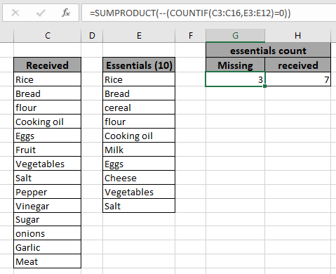
How to Count missing values in list in Excel

In this article, we will learn about how to look up missing values in the table in Excel using the formula shown in the above image.

Scenario:

For instance, we have a list of values and we need confirmation regarding the whereabouts of the required names in the list. Let's say we want to count the names of missing VIPs (VIP_names) in a guest list. For this, we will be considering the situation and suggest some formula to do the same. We will be using different function operations depending on the ease of the table_array.

Functions used and formula Syntax:

The following function will be in use. So get to know a little about, before using it.

We will construct a formula out of it. Firstly, the COUNTIF function takes each values one by one in criteria range and checks it in the range provided. SUMPRODUCT function returns the sum of TRUE values( as 1) and FALSE values (as 0) in the array.

Formula Syntax:

=SUMPRODUCT(--(COUNTIF(long_list,required)=0))

-- : operator used to convert TRUE values to FALSE values. Can be said as NOT function used for an array.

long_list : lookup list

required : required list

Example:

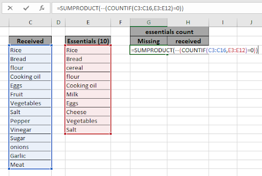
All of these might be confusing to understand. So, let's test this formula via running it on the example shown below. Here we have data having Price of products received on the dates. Here we need to find the count of items for all essentials items. So for that we have assigned 2 lists as the received list and essentials required in a column for the formula. Now we will use the below formula to get the count of products.

Use the formula:

=SUMPRODUCT(--(COUNTIF(C3:C16,E3:E12)=0))

Explanation for the formula:

COUNTIF function counts each item or cell in E3:E12 (essentials items) within received list (C3:C16).
=0 extracts the list of essentials in array.
-- operator returns the negation of the array i.e. TRUE values to FALSE values.
SUMPRODUCT finds the sum which will be the count of essentials not in the received list.

Here the argument arrays to the function is given as cell reference.

As you can see the formula returns 3 as count of essential items not received. In a
list of 14 items received, there are still 3 items not in it.

If -- (negation operator is not used)

You must be wondering what this negation (--) operator does. Let's use the above formula without using the negation (--) character.

Syntax of formula:

=SUMPRODUCT((COUNTIF(C3:C16,E3:E12)=0))

This formula returns 7 which is the count of essential items in received items. This formula only works when there is no duplicate item in both list. Check duplicates before using the formula.

As you can see from the above formula returns the Count missing values in list. Here are some observational results using the above formula used.

Notes:

Use the cell references to the accurate cells or the results will be changed.
The COUNTIF function supports Wildcards ( * , ? ) which helps in extracting values having phrases.
(--) operator negates the signs 1s to 0s and 0s to 1s.
The array argument to the function can be given as cell reference or named ranges.
You can customize these formulas as required using other excel function.
The function returns the sum of the values satisfying all the conditions.

Hope this article about How to Count missing values in list in Excel is explanatory. Find more articles on COUNTIF formulas here. If you liked our blogs, share it with your fristarts on Facebook. And also you can follow us on Twitter and Facebook. We would love to hear from you, do let us know how we can improve, complement or innovate our work and make it better for you. Write to us at info@exceltip.com.

Related Articles

IF with AND function : Implementation of logic IF function with AND function to extract results having criteria in Excel.

IF with OR function : Implementation of logic IF function with OR function to extract results having criteria in excel data.

How to use nested IF function : nested IF function operates on data having multiple criteria. The use of repeated IF function is nested IF excel formula.

SUMIFS using AND-OR logic : Get the sum of numbers having multiple criteria applied using logic AND-OR excel function.

Minimum value using IF function : Get the minimum value using the excel IF function and MIN function on array data.

How to use wildcards in excel : Count cells matching phrases using the wildcards in excel

Popular Articles

50 Excel Shortcut to Increase Your Productivity : Get faster at your task. These 50 shortcuts will make you work even faster on Excel.

The VLOOKUP Function in Excel : This is one of the most used and popular functions of excel that is used to lookup value from different ranges and sheets.

COUNTIF in Excel 2016 : Count values with conditions using this amazing function. You don't need to filter your data to count specific values. Countif function is essential to prepare your dashboard.

How to Use SUMIF Function in Excel : This is another dashboard essential function. This helps you sum up values on specific conditions.