In this article, you will learn how to create dynamic drop down list; after the selection from first list, the second drop down list will be dynamically updated. We will use INDIRECT function & Name Manager.
The dynamic drop down list will be helpful for the end user to select the item from the drop down list that belongs to the first list.
With the use of Data Validation feature in Excel, you can create your own custom error message when the user enters the information which is not predefined.
In this article we will use INDIRECT function & Name Manager.
INDIRECT: Returns the reference specified by a text string.
Syntax: =INDIRECT(ref_text,A1)
ref_text is a reference to a cell. If ref_text is not a valid cell reference, then INDIRECT function will return #REF error.
The second argument A1 refers to a logical value that specifies type of reference is contained in the cell ref_text.
If a1 is TRUE or omitted then ref_text is determined as A1-style reference.
If a1 is FALSE then ref_text is determined as R1C1 style reference.
Example: If value in cell A1 contains 10, B1 contains A1 & we use INDIRECT function in cell C1=INDIRECT(B1), then the result would be 10.
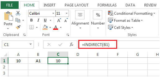
Let us take an example:
We have Cars data i.e. their Make & Model
The idea is to select the Make of the car, & Model of the car should be dynamically updated & available for selection.

The very first step is to make list of Models
Select the range E2:H6 & press CTRL + SHIFT + F3 (shortcut for creating multiple lists)
The Create Names from Selection window will appear
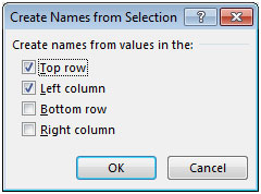
Make the Top row option checked & click on OK

Press CTRL + F3 to open Name Manager, and you will find the list of Car Make

Here, the only problem is the list created contains the blanks like cell E6, F5, F6 & so on.
We can easily remove the blanks using GO TO command.
Select the range E2:H6 & press F5 key on the keyboard to open the GO TO command
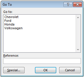
Click on Special & select Blanks then click on OK.
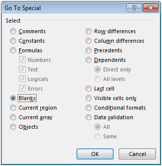
This will select all the blank cells in the selected range.
Right click or press CTRL + - (dash)
Select Shift cells up & then click OK
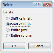
You can check the correct name list using CTRL + F3

Now, the empty cells have been removed.
Click on range B2:B5
Click on Data tab
From Data Tools group, select Data Validation option
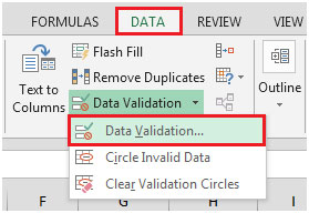
Or use ALT + D + L shortcut keys for Data Validation
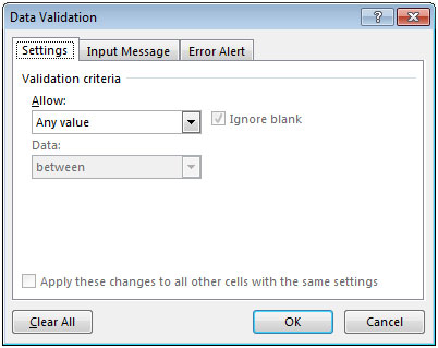
In Settings group, click on Allow & select List.
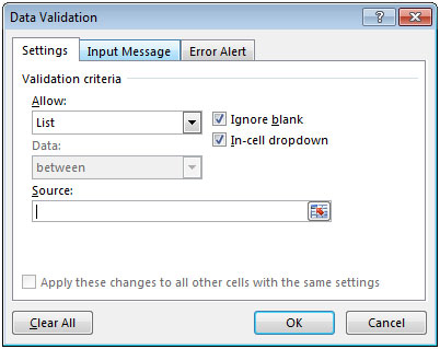
In Source enter the formula as =INDIRECT(A2)&click on Ok button

Click on cell B2 to see the options available for selection.
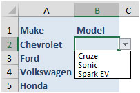
You can select the Model dependent on the value entered in column A.
In this way, you can create dynamic dropdown lists.
The applications/code on this site are distributed as is and without warranties or liability. In no event shall the owner of the copyrights, or the authors of the applications/code be liable for any loss of profit, any problems or any damage resulting from the use or evaluation of the applications/code.