How to Find Average of the Last 3 Non-zero Values in Microsoft Excel 2010

In this article, we will learn How to Find the Average of the Last 3 Non-zero Values in Microsoft Excel 2010.

Scenario :

When working with average computation on data. We usually come across the situation of considering zero or non-zero values. This is done as Average of of numbers just not only depends on the value, it also depends on the number of values considered. Average of n numbers is equal to the sum of numbers upon n.

Average of n values = Sum of n values / n

Here the criteria is, where we only have to considered 3 values which have non zero values. Let's understand this formula using different functions.

AVERAGE of last 3 non zero values in Excel

We use the AVERAGE function, IF , ROW & LARGE function. The combination of these will result in the average.

AVERAGE function can be used to find the average value or arithmetic mean of values in a selected range of cells.

Syntax: 

=AVERAGE(number1,number2,...)

number1, number2,……number n are numeric values.They can be numbers or names, arrays, of references that contain numbers.

The IF function checks if a condition you specify is TRUE or FALSE. If the condition returns TRUE then it returns preset value, and if the condition returns FALSE then it returns another preset value.

Syntax :

= IF(logical_test,value_if_true,value_if_false)

logical_test: Logical test will test the condition or criteria.If condition meets then it returns true, and if the condition does not meet then it returns false.

value_if_true: The value that you want to be returned if this argument returns TRUE.

value_if_false: The value that you want to be returned if this argument returns FALSE

ROW function Returns the row number of a reference.

Syntax: 

=ROW(reference)

Reference : It is a reference to a cell or range of cells.

LARGE : Returns the kth largest value in a data set. For example, the second largest number from a list of 10 items.

Syntax:

=LARGE(array,k)

array: It is an array or range of cells in a list of data for which you want to find the kth largest value.

k: It is the kth position from largest value to return in the array or range of cells.

Example :

All of these might be confusing to understand. Let's understand how to use the formula using an example. Here we have an example to demonstrate the average of values. But the condition is we don't want to include zero value.

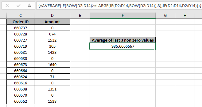
Use the formula:

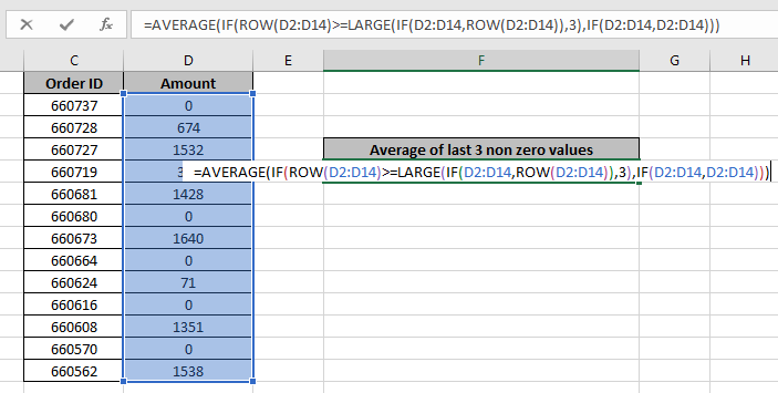
Donot press just Enter, Use Ctrl + Shift + Enter to get the average. Just choosing the Enter key option will result in #NUM error. So beware, This is done when an array of values is passed from inner function to outer function in a formula.

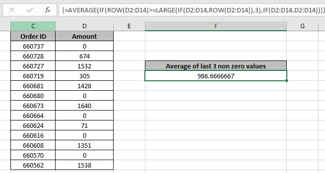
It is the average of 71, 1351 & 1538. Now you know how to do this so you perform the below example shown below.

Alternate way:

Here we have 5 ranges of numbers and We need to find the find the average of the top 3 values for all ranges.

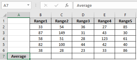
We need to find the average using the below formula

Use the formula:

Explanation:

The LARGE function gets the top 3 values of the range ( B1:B6 ). The Large function returns the values { 87 , 82 , 58 }. Now AVERAGE of these values is calculated using the AVERAGE function

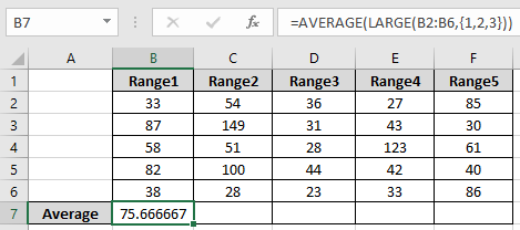
As you can see the formula returns the average for first array

Now use the same formula for other ranges using the Ctrl + R or drag right option in excel.

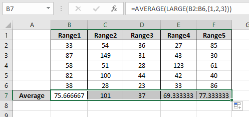
Here we have the average for all the ranges. You can perform more average function function using the AVERAGEIF, AVERAGEA, AVERAGEIFS & AGGREGATE functions here.

Here are all the observational notes regarding using the formula.

Notes:

1. Use Ctrl +Shift + Enter to get the If function working for arrays.
2. You can check the parts of the result, select the part of the formula and use windows + f9  from your windows pcs or laptop.
3. The function returns #VALUE! criteria if no value matches the given criteria.
4. Different Criteria inside formula is accepted, such as equals to (=), less than (<) , less than or equals to (<=) , greater than or equals to (>=) , greater than (>) & not equals to (<>).

In this way, we learnt How to Find the Average of the Last 3 Non-zero Values in Microsoft Excel 2010. You can use these functions in Excel 2016, 2013 and 2010. Find more articles on Mathematical operation and formulation with different criteria. If you liked our blogs, share it with your friends on Facebook. And also you can follow us on Twitter and Facebook. We would love to hear from you, do let us know how we can improve, complement or innovate our work and make it better for you. Write us at info@exceltip.com

Related Articles

How To Highlight Cells Above and Below Average Value : highlight values which are above or below the average value using the conditional formatting in Excel.

Ignore zero in the Average of numbers : calculate the average of numbers in the array ignoring zeros using AVERAGEIF function in Excel.

Calculate Weighted Average : find the average of values having different weight using SUMPRODUCT function in Excel.

Average Difference between lists : calculate the difference in average of two different lists. Learn more about how to calculate average using basic mathematical average formula.

Average numbers if not blank in Excel : extract average of values if cell is not blank in excel.

AVERAGE of top 3 scores in a list in excel : Find the average of numbers with criteria as highest 3 numbers from the list in Excel

Popular Articles:

How to use the IF Function in Excel : The IF statement in Excel checks the condition and returns a specific value if the condition is TRUE or returns another specific value if FALSE.

How to use the VLOOKUP Function in Excel : This is one of the most used and popular functions of excel that is used to lookup value from different ranges and sheets.

How to use the COUNTIF Function in Excel : Count values with conditions using this amazing function. You don't need to filter your data to count specific values. Countif function is essential to prepare your dashboard.

How to use the SUMIF Function in Excel : This is another dashboard essential function. This helps you sum up values on specific conditions.