How to Get Name of Day from Date Using VLOOKUP in Microsoft Excel 2010

In this article, we will learn How to Get Name of Day from Date Using VLOOKUP in Microsoft Excel 2010.

In this article, we will learn about how to use VLOOKUP function in Excel to find the data by Date.

VLOOKUP just searches for the row of a given value in the first column of a table and returns asked column’s value in that row.

Syntax:

Lookup_date:  The date by which you want to search in the first column of Table Array.

Table_array: The Table in which you want to look up/search

col_index_number:  The column number in Table Array from which you want to fetch results.

[range_lookup]: FALSE if you want to search for exact value, TRUE if you want an approximate Date match.

Here we know LOOKUP value is by Date

Let’s understand this function using it an example.

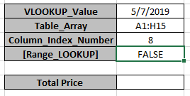
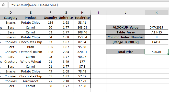
Here we have a Data Table and Vlookup Information and we need to find the Total Price by the date 5/7/2019.

To find the value, use the Vlookup formula

Explanation

The Formula looks up for the date in K3 cell in the table A1:H15.

Now once the date is found by the formula, It will lookup 8th column of the Table_array.

As the Last argument is False it will look for exact Date Match.

As you can see here, the formula has the Total price for the provided date.

Another Example

Scenario:

We have a long table entry of Products and there are blank cells between the values. We need to find the last entry value and date associated with it.

We will be using the LOOKUP function. Let's first get some knowledge about the function.

LOOKUP function finds the estimated value in the range and returns the value from the range or its corresponding value.

Syntax:

lookup_value: value to look up for

lookup_vector: array where the function looks for the lookup_value.

[result vector]:[optional] if the return array is different from the lookup array.

But here we will be using its one of the attributes of the LOOKUP function i.e. if LOOKUP function can't find an exact match, it will match with just the previous value. It returns the last found value for the previous value. So we will be using the below syntax.

Generic Formula:

list : lookup list

date_range : date value to be returned from the range

Example

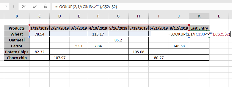
Here we have products delivered with its date and amount and we need to find the last delivered product date for each product.

So here we have some blank cells between the value entries.

Formula:

C$2:J$2 : fixed date_range

Explanation:

• <>"" this pattern with a list returns array of TRUEs and FALSEs. TRUE value corresponding to existing value and FALSE value corresponding to blank cells.
• TRUE value is considered as a numerical value 1 and FALSE value as 0.
• LOOKUP function looks up for the numerical value 2 in the array of 1s and 0s.
• So when the function doesn't find the value 2. So it looks backward in the array for the less closest value to 2 which is 1 here.
• The function returns the date related to last entry.

Press Enter to get the results.

As you can see the 10-Apr is the last entry date for the Wheat product.

Now copy the formula to other cells using the shortcut Ctrl + D or drag down cell option from right bottom of the cell.

As you can see, the function returns the value as required. You can customize Excel functions as required.

Here we have observational notes for using the formula.

Notes: 

1. The formula returns #NA error if no match is found in the array.
2. The formula checks the lookup value first and then looks up for the just previous value, if the lookup value is not found.
3. All excel formula always returns the first value found in the table array.
4. The above explained formula, lookup for the last entry and returns date related to the corresponding last value.

Hope this article about How To Find The Last Used Cell in One Column in Microsoft Excel 2010 is explanatory. Find more articles on reference formulas here. If you liked our blogs, share it with your fristarts on Facebook. And also you can follow us on Twitter and Facebook. We would love to hear from you, do let us know how we can improve, complement or innovate our work and make it better for you. Write to us at info@exceltip.com.

Related Articles

Use INDEX and MATCH to Lookup Value : INDEX & MATCH function to look up value as required.

SUM range with INDEX in Excel : Use INDEX function to find the SUM of the values as required.

How to use the SUM function in Excel : Find the SUM of numbers using the SUM function explained with example.

How to use the INDEX function in Excel : Find the INDEX of array using the INDEX function explained with example.

How to use the MATCH function in Excel : Find the MATCH in the array using the INDEX value inside MATCH function explained with example.

How to use LOOKUP function in Excel : Find the lookup value in the array using the LOOKUP function explained with example.

How to use the VLOOKUP function in Excel : Find the lookup value in the array using the VLOOKUP function explained with example.

How to use the HLOOKUP function in Excel : Find the lookup value in the array using the HLOOKUP function explained with example.

Popular Articles :

How to use the IF Function in Excel : The IF statement in Excel checks the condition and returns a specific value if the condition is TRUE or returns another specific value if FALSE.

How to use the VLOOKUP Function in Excel : This is one of the most used and popular functions of excel that is used to lookup value from different ranges and sheets.

How to Use SUMIF Function in Excel : This is another dashboard essential function. This helps you sum up values on specific conditions.

How to use the COUNTIF Function in Excel : Count values with conditions using this amazing function. You don't need to filter your data to count specific values. Countif function is essential to prepare your dashboard.