How to Use Conditional Summing for Specific Conditions

In this article, we will learn How to Use Conditional Summing for Specific Conditions.

Scenario:

In simple words, when working with a long scattered dataset, sometimes we need to find the sum of numbers with some criteria over it. For example, finding the sum of salaries in a particular department or having multiple criterias over date, names, department or can even numbers data like salaries below value or quantity above value. For this you usually use the SUMPRODUCT or SUMIFS function. But you wouldn't believe, you perform the same function with Excel basic function IF function.

How to solve the problem?

You must be thinking how is this possible, to perform logical operations over table arrays using IF function. IF function in excel is very useful, It will get you through some difficult tasks in Excel or any other coding languages. IF function tests conditions on array corresponding to required values and returns the result as array corresponding to True conditions as 1 and False as 0

For this problem, we will be using the following functions :

We will be requiring these above functions and some basic sense of data operation. logical conditions on arrays can be applied using logical operators. These logic operators work on text and numbers both. Below here is the generic formula. { } curly braces is the magic tool to perform array formulas with IF function.

Generic formula:

{ = SUM ( IF ( (logical_1) * (logical_2) * …* (logical_n) , sum_array ) ) }

Note: For curly braces ( { } ) Use Ctrl + Shift + Enter when working with arrays or ranges in Excel. This will generate Curly Braces on the formula by default. DO NOT try to hard code curly braces characters.

Logical 1 : tests condition 1 on array 1

Logical 2 : tests condition 2 on array 2 and so on

sum_array : array, operation sum is performed

Example :

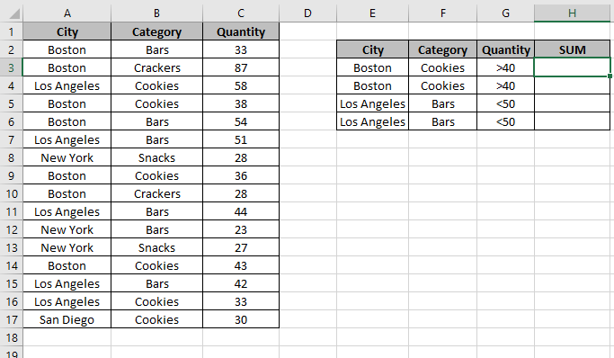
All of these might be confusing to understand. So, let's test this formula via running it on the example shown below. Here we have data of delivered products to different cities along with corresponding category fields and quantities. Here we have the data and we need to find the quantity of cookies sent to Boston where the quantity be greater than 40.

Data table and criteria table are shown in the above image. For understanding purpose we used named ranges for the used arrays. Named ranges are listed below.

Here :

City defined for array A2:A17.

Category defined for array B2:A17.

Quantity defined for array C2:C17.

Now you are ready to get the desired result using the below formula.

Use the formula :

{ = SUM ( IF ( (City="Boston") * (Category="Cookies") * (Quantity>40) , Quantity)) }

Explanation :

City ="Boston" : checks the values in city range to match with "Boston".
Category="Cookies" : checks the values in Category range to match with "Cookies".
Quantity > 40 : checks the values in Quantity range to ma
Quantity be array where sum is required.
IF function checks all criteria and asterisk char (*) multiples all the array results.

= SUM ( IF ( { 0 ; 0 ; 0 ; 0 ; 0 ; 0 ; 0 ; 0 ; 0 ; 0 ; 0 ; 0 ; 1 ; 0 ; 0 ; 0 } , { 33 ; 87 ; 58 ; 38 ; 54 ; 51 ; 28 ; 36 ; 28 ; 44 ; 23 ; 27 ; 43 ; 42 ; 33 ; 30 } ) )

Now IF function only returns the quantities corresponding to the 1s and rest are ignored.
SUM function returns the SUM.

Now the quantity corresponding to 1’s only adds up to get the result.

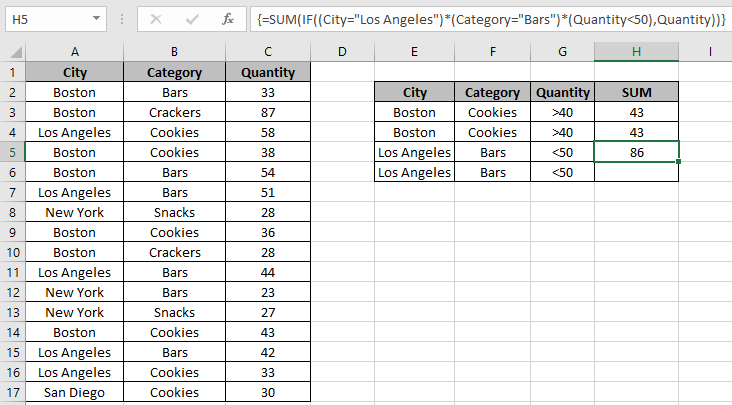
As you can see, quantity 43 is returned but there are three cookie orders delivered to "Boston" having quantity 38, 36 and 43. We needed a sum of quantity where quantity be above 40. So the formula returns 43 only. Now use other criteria to get the SUM Quantity for City : "Los Angeles" & Category : "Bars" & Quantity be less than 50.

Use the formula

{ = SUM ( IF ( ( City = "Los Angeles") * (Category="Bars") * (Quantity < 50), Quantity ) ) }

As you can see, the formula returns the values 86 as result. Which is the sum of 2 orders satisfying the conditions having quantity 44 & 42. You can use nested IF, SUMIFS or SUMPRODUCT function in Excel to solve the same problem. We can recheck the result using the SUMPRODUCT function

Use of SUMPRODUCT function:

SUMPRODUCT function returns the sum of corresponding values in the array. So we will get the arrays to returns 1s a the True statement values and 0s to the False statement values. So last sum will be corresponding where all statements stands True.

Use the formula:

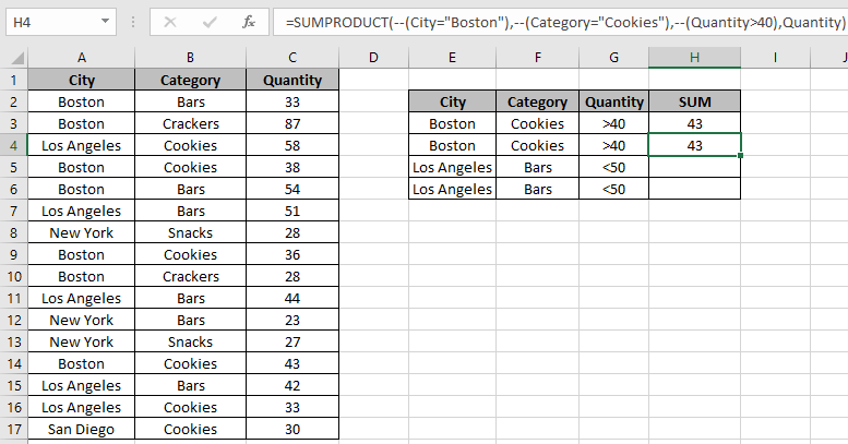
= SUMPRODUCT ( -- (City = "Boston") , -- (Category = "Cookies") , -- (Quantity > 40) , Quantity )

-- : operation used to convert all TRUEs to 1s and False to 0.

SUMPRODUCT function rechecks the SUM of quantity returned by the SUM and IF function explained above.

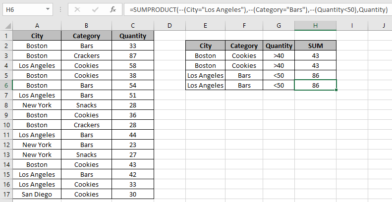
Similarly for the second example the result stands the same.

As you can see SUMPRODUCT function can perform the same task.

Here are all the observational notes regarding using the formula.

Notes:

The sum_array in the formula only works with numbers.
If the formula returns #VALUE error, check for the curly braces must be present in the formula as shown in the examples in the article.
Negation (--) char changes values, TRUEs or 1s to FALSEs or 0s and FALSEs or 0s to TRUEs or 1s .
Operations like equals to ( = ), less than equal to ( <= ), greater than ( > ) or not equals to ( <> ) can be performed within a formula applied, with numbers only.

Hope this article about How to Use Conditional Summing for Specific Conditions in Excel is explanatory. Find more articles on Summing formulas here. If you liked our blogs, share it with your fristarts on Facebook. And also you can follow us on Twitter and Facebook. We would love to hear from you, do let us know how we can improve, complement or innovate our work and make it better for you. Write us at info@exceltip.com

Related Articles :

How to use the SUMPRODUCT function in Excel: Returns the SUM after multiplication of values in multiple arrays in excel.

SUM if date is between : Returns the SUM of values between given dates or period in excel.

Sum if date is greater than given date: Returns the SUM of values after the given date or period in excel.

2 Ways to Sum by Month in Excel: Returns the SUM of values within a given specific month in excel.

How to Sum Multiple Columns with Condition: Returns the SUM of values across multiple columns having condition in excel.

Popular Articles :

How to use the IF Function in Excel : The IF statement in Excel checks the condition and returns a specific value if the condition is TRUE or returns another specific value if FALSE.

How to use the VLOOKUP Function in Excel : This is one of the most used and popular functions of excel that is used to lookup value from different ranges and sheets.

How to Use SUMIF Function in Excel : This is another dashboard essential function. This helps you sum up values on specific conditions.

How to use the COUNTIF Function in Excel : Count values with conditions using this amazing function. You don't need to filter your data to count specific values. Countif function is essential to prepare your dashboard.