In this article, we will learn How to Lookup and Reference functions in Excel.

If you have multiple excel tables and you want to do a dynamic VLOOKUP Function from these tables, you will need to use the INDIRECT function. In this article we will learn how easily you can change your lookup table by just changing the name of the lookup table in a cell.
Generic Formula for Dynamic Table VLOOKUP
| =VLOOKUP(lookup_value, INDIRECT("TableName"), col_index,0) |
Lookup_value: The value you are looking for.
TableName: The table in which you want to look for the lookup value.
Col_Index: The column number from which you want to retrieve data.
Let's hope on to an example to see how it works.
Example: Create A Dynamic Lookup Formula To Look Up From Selected Table

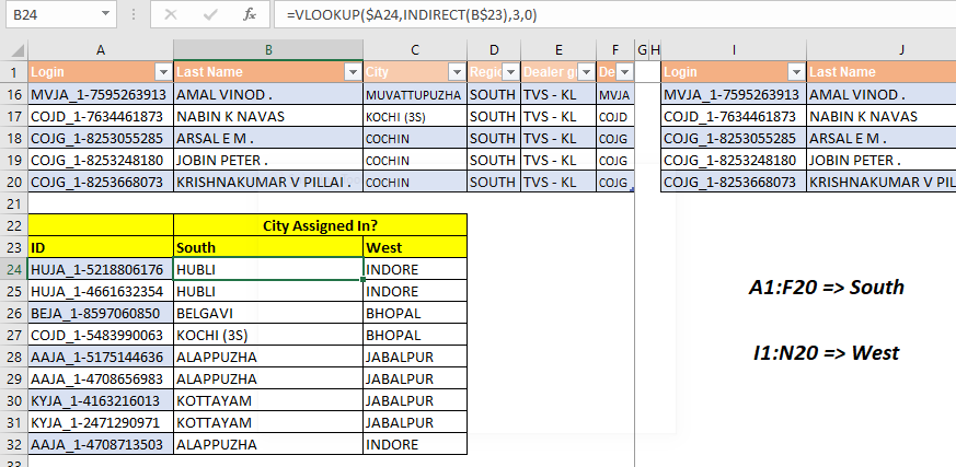
Here we have two tables of the same employees. First table is named South and contains data of employees assigned in South cities. Second table is named West and contains the details of the same employees when assigned in cities of West.
Now we need to get the cities of employees at the same place from both regions.
As you can see in the image, we have prepared a table down. It contains the ids of employees. We need to get the cities from South and West using one single formula.
Apply above generic formula to write this formula for dynamic VLOOKUP:
| =VLOOKUP($A24,INDIRECT(B$23),3,0) |
We have locked the references using $ sign so that when we copy the formula it takes the right references.
| If you aren't familiar with reference locking or absolution, you learn it here. It is really important if you want to master Excel. |
Write the above formula in cell B24, copy in whole range.

You can see that it has looked up the city of South from the South table and City of West from the West table, dynamically. We did not need to change anything in the formula.
How does it work?
It is a basic VLOOKUP formula with only difference of INDIRECT function. As you know that INDIRECT function converts any text reference into actual reference, we use the same ability of INDIRECT function here.
It is important that you use an Excel Table or name your tables using named ranges.
In B24, we have formula VLOOKUP($A24,INDIRECT(B$23),3,0). This resolves to VLOOKUP($A24,INDIRECT("South"),3,0). Now indirect converts "South" into actual table reference (we have named the first table as South. Hence the formula is now VLOOKUP($A24,South,3,0). Now VLOOKUP simply looks up in the SOUTH table.
When we copy formulas in C24, the formula becomes VLOOKUP($A24,INDIRECT(C$23),3,0). Now C23 contains "West". Hence the formula will ultimately resolve to VLOOKUP($A24,West,3,0). And VLOOKUP gets the value from the West table this time.
Hope this article about How to Lookup and Reference function in Excel is explanatory. Find more articles on lookup formulas and related Excel formulas here. If you liked our blogs, share it with your friends on Facebook. And also you can follow us on Twitter and Facebook. We would love to hear from you, do let us know how we can improve, complement or innovate our work and make it better for you. Write to us at info@exceltip.com.
Related Articles:
Use INDEX and MATCH to Lookup Value : The INDEX-MATCH formula is used to lookup dynamically and precisely a value in a given table. This is an alternative to the VLOOKUP function and it overcomes the shortcomings of the VLOOKUP function.
Use VLOOKUP from Two or More Lookup Tables : To lookup from multiple tables we can take an IFERROR approach. To lookup from multiple tables, it takes the error as a switch for the next table. Another method can be an If approach.
How to do Case Sensitive Lookup in Excel : The excel's VLOOKUP function isn’t case sensitive and it will return the first matched value from the list. INDEX-MATCH is no exception but it can be modified to make it case sensitive. Let’s see how…
Lookup Frequently Appearing Text with Criteria in Excel : The lookup most frequently appears in text in a range we use the INDEX-MATCH with MODE function. Here's the method.
Popular Articles :
How to use the IF Function in Excel : The IF statement in Excel checks the condition and returns a specific value if the condition is TRUE or returns another specific value if FALSE.
How to use the VLOOKUP Function in Excel : This is one of the most used and popular functions of excel that is used to lookup value from different ranges and sheets.
How to Use SUMIF Function in Excel : This is another dashboard essential function. This helps you sum up values on specific conditions.
How to use the COUNTIF Function in Excel : Count values with conditions using this amazing function. You don't need to filter your data to count specific values. Countif function is essential to prepare your dashboard.
The applications/code on this site are distributed as is and without warranties or liability. In no event shall the owner of the copyrights, or the authors of the applications/code be liable for any loss of profit, any problems or any damage resulting from the use or evaluation of the applications/code.