In this article, we will learn Multiple ways to change the text case in Excel.
Scenario:
Working on text columns like names column or address column in data, gets us into some problems when we need to get the columns in correct format as required. Here's a whole category of Excel functions to deal with text, and these three will help us to change the text cases.
Common usage text functions to change text cases
The LOWER function in excel is used to make text of lower case
LOWER function syntax
| =LOWER(Text) |
The UPPER function in excel is used to capitalize all letters of a string,
UPPER function syntax
| =UPPER(text) |
The PROPER function in excel is used to make text of Proper Case or say Title Case. The function capitalises the first alphabet of each word in a cell.
PROPER function syntax
| =PROPER(text) |
Note: input text directly in quotes like "value" or input value in some cell like A2 cell and use cell reference in function to input value as argument.
Example :
All of these might be confusing to understand. Let's understand how to use the function using an example. Here we’re going to look at using Excel functions, flash fill, power query, DAX and power pivot to change the case of our text data. There’s a whole category of Excel functions to deal with text, and these three will help us to change the text case.
LOWER Excel Worksheet Function

| =LOWER(A2) |
The LOWER function takes one argument which is the bit of Text we want to change into lower case letters. The function will evaluate to text that is all lower case.
UPPER Excel Worksheet Function

| =UPPER(A2) |
The UPPER function takes one argument which is the bit of Text we want to change into upper case letters. The function will evaluate to text that is all upper case.
PROPER Excel Worksheet Function.
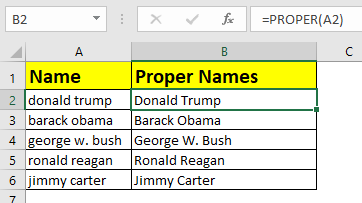
| =PROPER(A2) |
The PROPER function takes one argument which is the bit of Text we want to change into the proper case. The function will evaluate to text that is all proper case where each word starts with a capital letter and is followed by lower case letters.
Copy And Paste Formulas As Values
After using the Excel formulas to change the case of our text, we may want to convert these to values.
This can be done by copying the range of formulas and pasting them as values with the paste special command.
Press Ctrl + C to copy the range of cells > press Ctrl + Alt + V to paste special > choose Values from the paste options.
Using Flash Fill To Change Text Case
Flash fill is a tool in Excel that helps with simple data transformations. We only need to provide a couple examples of the results we want, and flash fill will fill in the rest.

Flash fill can only be used directly to the right of the data we’re trying to transform. We need to type out a couple of examples of the results we want. When Excel has enough examples to figure out the pattern, it will show the suggested data in a light grey font. We can accept this suggested filled data by pressing Enter.
We can also access flash fill from the ribbon. Enter the example data > highlight both the examples and cells that need to be filled > go to the Data tab > press the Flash Fill command found in the Data Tools section.
We can also use the keyboard shortcut Ctrl + E for flash fill.
Flash fill will work for many types of simple data transformations including changing text between lower case, upper case and proper case.
Using Power Query To Change Text Case
Power query is all about data transformation, so it’s sure there is a way to change the case of text in this tool.
With power query we can transform the case into lower, upper and proper case.

Select the data we want to transform > go to the Data tab > select From Table/Range. This will open up the power query editor where we can apply our text case transformations.
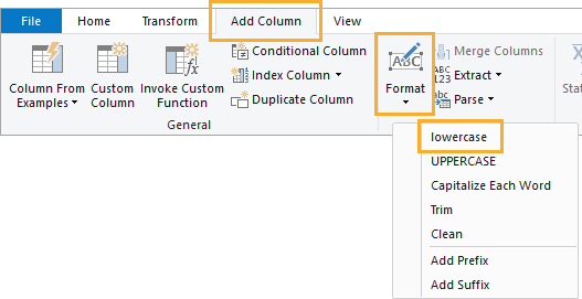
Select the column containing the data we want to transform > go to the Add Column tab > select Format > select lowercase from the menu.
| = Table.AddColumn(#"Changed Type", "lowercase", each Text.Lower([Name]), type text) |
This will create a new column with all text converted to lower case letters using the Text.Lower power query function.
Text.Upper Power Query Function
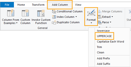
Select the column containing the data we want to transform > go to the Add Column tab > select Format > select UPPERCASE from the menu.
| = Table.AddColumn(#"Changed Type", "UPPERCASE", each Text.Upper([Name]), type text) |
This will create a new column with all text converted to upper case letters using the Text.Upper power query function.

Select the column containing the data we want to transform > go to the Add Column tab > select Format > select Capitalize Each Word from the menu.
| = Table.AddColumn(#"Changed Type", "Capitalize Each Word", each Text.Proper([Name]), type text) |
This will create a new column with all text converted to proper case lettering, where each word is capitalized, using the Text.Proper power query function.
Using DAX Formulas To Change Text Case
When we think of pivot tables, we generally think of summarizing numerical data. But pivot tables can also summarize text data when we use the data model and DAX formulas. There are even DAX formulas to change the text case before we summarize it.

First, we need to create a pivot table with our text data. Select the data to be converted > go to the Insert tab > select PivotTable from the tables section.
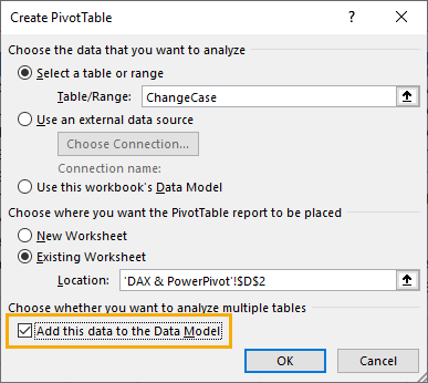
In the Create PivotTable dialog box menu, check the option to Add this data to the Data Model. This will allow us to use the necessary DAX formula to transform our text case.
Creating a DAX formula in our pivot table can be done by adding a measure. Right click on the table in the PivotTable Fields window and select Add Measure from the menu.
This will open up the Measure dialog box, where we can create our DAX formulas.
LOWER DAX Function

| =CONCATENATEX( ChangeCase, LOWER( ChangeCase[Mixed Case] ), ", ") |
We can enter the above formula into the Measure editor. Just like the Excel worksheet functions, there is a DAX function to convert text to lower case.
However, in order for the expression to be a valid measure, it will need to be wrapped in a text aggregating function like CONCATENATEX. This is because measures need to evaluate to a single value and the LOWER DAX function does not do this on it’s own. The CONCATENATEX function will aggregate the results of the LOWER function into a single value.
We can then add the original column of text into the Rows and the new Lower Case measure into the Values area of the pivot table to produce our transformed text values.
Notice the grand total of the pivot table contains all the names in lower case text separated by a comma and space character. We can hide this part by going to the Table Tools Design tab > Grand Totals > selecting Off for Rows and Columns.
UPPER DAX Function

| =CONCATENATEX( ChangeCase, UPPER( ChangeCase[Mixed Case] ), ", ") |
Similarly, we can enter the above formula into the Measure editor to create our uppercase DAX formula. Just like the Excel worksheet functions, there is a DAX function to convert text to upper case.

Creating the pivot table to display the upper case text is the same process as with the lower case measure.
Missing PROPER DAX Function
We might try and create a similar DAX formula to create proper case text. But it turns out there is no function in DAX equivalent to the PROPER worksheet function.
Using Power Pivot Row Level Formulas To Change Text Case (Add-In option)
This method will also use pivot tables and the Data Model, but instead of DAX formulas we can create row level calculations using the Power Pivot add-in.
Power pivot formulas can be used to add new calculated columns in our data. Calculations in these columns happen for each row of data similar to our regular Excel worksheet functions.
Not every version of Excel has a power pivot available and you will need to enable the add-in before you can use it. To enable the power pivot add-in, go to the File tab > Options > go to the Add-ins tab > Manage COM Add-ins > press Go > check the box for Microsoft Power Pivot for Excel.
We will need to load our data into the data model. Select the data > go to the Power Pivot tab > press the Add to Data Model command.
This is the same data model as creating a pivot table and using the Add this data to the Data Model checkbox option. So if our data is already in the data model we can use the Manage data model option to create our power pivot calculations.
LOWER Power Pivot Function
Adding a new calculated column into the data model is easy. Select an empty cell in the column labelled Add Column then type out the above formula into the formula bar. You can even create references in the formula to other columns by clicking on them with the mouse cursor.
Press Enter to accept the new formula.
The formula will appear in each cell of the new column regardless of which cell was selected. This is because each row must use the same calculation within a calculated column.
We can also rename our new column by double clicking on the column heading. Then we can close the power pivot window to use our new calculated column.
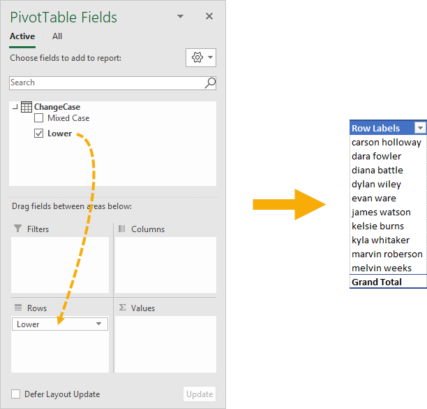
When we create a new pivot table with the data model, we will see the calculated column as a new available field in our table and we can add it into the Rows area of the pivot table. This will list out all the names in our data and they will all be lower case text.
We can do the same thing to create a calculated column that converts the text to upper case by adding a new calculated column with the above formula.

Again, we can then use this as a new field in any pivot table created from the data model.
Missing PROPER Power Pivot Function
Unfortunately, there is no power pivot function to convert text to proper case. So just like DAX, we won’t be able to do this in a similar fashion to the lowercase and uppercase power pivot methods.
Conclusions
There are many ways to change the case of any text data between lower, upper and proper case.
Here are all the observational notes using the formula in Excel
Notes :
Hope this article about Multiple ways to change text case in Excel is explanatory. Find more articles on calculating values and related Excel formulas here. If you liked our blogs, share it with your friends on Facebook. And also you can follow us on Twitter and Facebook. We would love to hear from you, do let us know how we can improve, complement or innovate our work and make it better for you. Write to us at info@exceltip.com.
Related Articles :
How to use the RIGHT function in Excel : Extract text from the RIGHT of the text just like the left function explained above in excel. Learn RIGHT function syntax and usage with an example
How to use the MID function in Excel : Extract text from the middle of the text just like the left or right function in excel. Learn MID function syntax and usage with an example
How to use the FIND function in Excel : find known text in the given cell and return the position of known text like the function usage explained above in excel. Learn FIND function syntax and usage with an example
How to use the SEARCH function in Excel : locate known text in the given cell and return the position of known text like the function usage explained above in excel. Learn SEARCh function syntax and usage with an example
How to Use TRIM function in Excel: The TRIM function is used to trim strings and clean any trailing or leading spaces from string. This helps us in the cleaning process of data a lot.
How to use the CLEAN function in Excel: Clean function is used to clean up unprintable characters from the string. This function is mostly used with the TRIM function to clean up imported foreign data.
Popular Articles :
50 Excel Shortcuts to Increase Your Productivity : Get faster at your tasks in Excel. These shortcuts will help you increase your work efficiency in Excel.
How to use the VLOOKUP Function in Excel : This is one of the most used and popular functions of excel that is used to lookup value from different ranges and sheets.
How to use the IF Function in Excel : The IF statement in Excel checks the condition and returns a specific value if the condition is TRUE or returns another specific value if FALSE.
How to use the SUMIF Function in Excel : This is another dashboard essential function. This helps you sum up values on specific conditions.
How to use the COUNTIF Function in Excel : Count values with conditions using this amazing function. You don't need to filter your data to count specific values. Countif function is essential to prepare your dashboard.
The applications/code on this site are distributed as is and without warranties or liability. In no event shall the owner of the copyrights, or the authors of the applications/code be liable for any loss of profit, any problems or any damage resulting from the use or evaluation of the applications/code.