In this article, you will learn how to show output with matching criteria using conditional formatting.
Q: I have a record set from column A to C (Code#, Account# and Amount). Now, I need a formula to highlight all the rows with Code between 40 & 50 in column A with Account in starting with 5 series in column B.
We have three columns of data & now, we want to highlight the rows which are matching the criteria.

Following snapshot shows the Output

We will use a combination of AND, OR & FIND functions in Conditional Formatting.
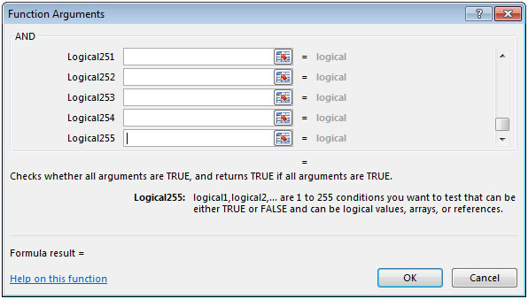
AND: Checks whether all arguments are TRUE, and returns TRUE if all the arguments are TRUE. If anyone is found to be FALSE, then AND function will returns FALSE.
Syntax =AND(logical1,logical2,...)
logical1: The first condition that you want to check
logical2: This is optional. You can add as many as 255 conditions at a time to evaluate to TRUE or FALSE.

The IF function checks if a condition you specify is TRUE or FALSE. If the condition returns TRUE then it returns preset value, and if the condition returns FALSE then it returns another preset value.
Syntax = IF(logical_test,value_if_true,value_if_false)
logical_test: Logical test will test the condition or criteria. If condition meets then it returns the preset value, and if the condition does not meet then it returns another preset value.
value_if_true: The value that you want to be returned if this argument returns TRUE.
value_if_false: The value that you want to be returned if this argument returns FALSE
FIND: Returns the starting position of one text string within another text string. FIND is a case sensitive.
Syntax: =FIND(find_text,within_text,start_num)
find_text: The text that you want to find.
within_text: Itis the text in which you want to search.
start_num: This is optional. It is the number in the string from which you want to extract data.
To get the output, select range A4:C20
From Home tab, click on Conditional Formatting & select New Rule
Or press ALT + O + D shortcut
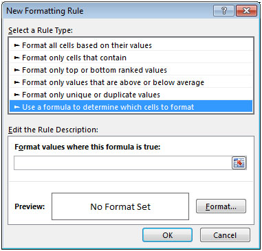
This will open New Formatting Rule Manager
Select “Use a formula to determine which cells to format”

Enter the formula as =AND(OR($A4>=40,$A4<=50),FIND("5",$B4,1)=1)

Click on Format & select the color & click on OK twice.

In this way, we can highlight the rows which are matching the criteria.
The applications/code on this site are distributed as is and without warranties or liability. In no event shall the owner of the copyrights, or the authors of the applications/code be liable for any loss of profit, any problems or any damage resulting from the use or evaluation of the applications/code.