Sparkline’s in Microsoft Excel

In this article we will learn about how we can make the Sparkline in Microsoft Excel 2010 and 2013.

Spark lines are possibly the most appropriate way to analyze the data, this is a type of graph that shows variations of data in a single cell. If we do not have enough time to understand the data and want to quickly understand, Sparklines can immediately arrange the clear overview.

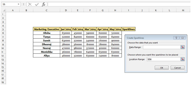
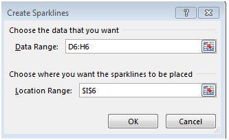
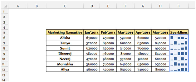
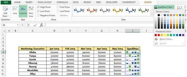
To create the Sparklines we use here Column Sparklines which are helpful to create mini charts placed in single cells, each representing a row or data in your selection.

Let’s take the examples and understand:

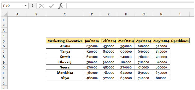
We are having sales data from the range C5 to H12. In which column C contains the name of Marketing Executive, Column D contains the sales amount of Jan’2014, Column E for Feb’2014, Column F for Mar’2014, Column G to Apr’2014 and Column H contains the sales amount of May’2014.

Select the cell I6.
Go to the Insert Tab in the ribbon, click on Column Sparklines in the Sparkline’s group.

Create Sparklines dialog box will appear.

Select the data range D6:H6, and select the location range I6 click ok and drag it down using the fill handle option from the bottom right corner of the cell.
Sparklines will create for each row.

After adding the spark lines in worksheet the design tab will appear.
The design tab contains buttons that edits the type, style, format of the sparklines.

Note: We cannot delete the Sparklines from a cell range by selecting the cell and then press the delete button.

To Delete the Sparklines follow below mentioned steps:-

Right click of the mouse.
Popup will get appear.
Click on the Sparklines clear the Sparklines group.

How to format Sparklines

Select the cell I6, Design tab will appear in the menu.
Select the marker color from the group of style, choose the green color for high point and choose the red color for low point.
We can make more analyzing to Sparklinesas per the requirement.

Note: If the Sparklines source data contain non-numeric value they are neglected while plotting the sparklines. If the data are having #N/A value they are ignored too. The Sparklines will show blank when data value would be zero or blank.