How to Square Root in Excel

In this article, we will learn How to Square Root in Excel.

SQRT function is used when we need to find the square root of a number in Excel.

The square root of x is referred to as x.

Square root operation in Mathematics.

The Root of a number is inverse of Power of the number.

Square of a number = Power(2) of a number

The square root of a number = power(½) of a number

y=x2 y =x

For example: under root or square root of 9 is 3. Square root of a value is used in many different aspects like calculating standard deviation using variance. Usually in Excel this function is used with other functions. Basically, when a number is divided by value and quotient comes out to be same as the value with zero remainder.

SQRT function in Excel

The function takes a single positive number and returns the square root of that number.

Syntax of SQRT function:

=SQRT(number)

Number : input number you want the square root of.

Example :

All of these might be confusing to understand. Let's understand how to use the function using an example. Here we have some values with which we can understand about the function results

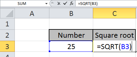
Use the formula to get the square root of the number in cell B3.

=SQRT(B3)

B3 : input number as a cell reference.

Press Enter to see the square root of 25. So the function will return 5 which is when 25 is divided by 5 quotient comes out to be 5 with remainder zero.

The square root of 25 is 5.

You can customize your formula with these basic functions. As you can see by using the mathematical function in Excel you can perform many exponents function. Please do find more articles on the mathematical formulation here.

In case you quickly want to calculate square root in Excel, you can use square root formula. In this article, we will learn on finding the square root of numbers in Excel.

The SQRT function can be used in the following versions of Microsoft Excel: Excel 2013, Excel 2010, Excel 2007, Excel 2003

Following is the snapshot of data:

In cell B2, the formula is
=SQRT(A2)& by dragging down the formula, we will get the squared in Excel

Few things to be considered:

Cell B8 shows #NUM! error in Excel.
The reason is if a negative number is entered in the number parameter, the SQRT function will return the #NUM! error.
Cell B9 shows #VALUE! error in Excel.
#VALUE! - Occurs if the supplied argument cannot be taken as a numeric value

In this way, we can calculate the square root in Excel.

Using POWER function

In mathematics, the power operator gets the power of a number.

33= 3 * 3 *3 = 27

3 raised to the power 3, says 3 multiplied by its own number three times is equals 27.

271/3= 33*(1/3)= 3

27 raised to the power (?), says which number gets multiplied 3 times to get 27, 3 is the answer. This is called finding the root of a number.

POWER function calculates the power of a number.

Syntax:

=POWER ( number, power)

For example: IF you wish to get the power of 4 raised to 3

Write the formula in the cell =POWER(4,3)

Let’s learn this through an example shown below.

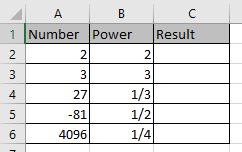
Here we have numbers in one column and power of the numbers in the second column.

Use the formula to get the POWER

=POWER(A2,B2)

Press Enter and copy the formula in other cells using Ctrl + D shortcut.

As you can see the formula returns #NUM error when we calculate the root of a negative number.

Notes:

The number can be positive decimal and positive integer value.
The function returns the #VALUE! Error, if the argument to the function is non numeric.
The function returns the #NUM! Error, if the argument to the function is less than zero. Use the ABS function to the input number to get the square root of a positive number.
Operations like equals to ( = ), less than equal to ( <= ), greater than ( > ) or not equals to ( <> ) can be performed within a formula applied, with numbers only.

Hope this article about How to Square Root in Excel is explanatory. Find more articles on mathematical formulas and related Excel functions here. If you liked our blogs, share it with your friends on Facebook. And also you can follow us on Twitter and Facebook. We would love to hear from you, do let us know how we can improve, complement or innovate our work and make it better for you. Write to us at info@exceltip.com.

Related Articles :

How to use the SQRT Function in Excel : The SQRT Function in Excel performs the under root or square root operation of the input positive number using the SQRT function in Excel.

How to use the POWER function in Excel : ThePOWER function in Excel performs the power operation (which is number raised to the power value) on the input number using the POWER function in Excel

How to use the ISEVEN function in Excel | returns the TRUE logic value if the number is EVEN using the ISEVEN function in Excel.

How to use the ISODD function in Excel | returns the TRUE logic value if the number is ODD using the ISODD function in Excel.

Popular Articles :

How to use the IF Function in Excel : The IF statement in Excel checks the condition and returns a specific value if the condition is TRUE or returns another specific value if FALSE.

How to use the VLOOKUP Function in Excel : This is one of the most used and popular functions of excel that is used to lookup value from different ranges and sheets.

How to Use SUMIF Function in Excel : This is another dashboard essential function. This helps you sum up values on specific conditions.

How to use the COUNTIF Function in Excel : Count values with conditions using this amazing function. You don't need to filter your data to count specific values. Countif function is essential to prepare your dashboard.