How to Use of Conditional Formatting in Microsoft Excel

To color rows based on text criteria we use the “Conditional Formatting” option. This option is available in the “Home Tab” in the “Styles” group in Microsoft Excel.

Conditional Formatting: - To highlight the specific cells or range on the basis of text criteria's, number criteria's etc.

 
Let’s take an example to understand the use of Conditional Formatting in Excel:-

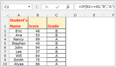
We have data in range A1:A10. Column C contains the grades. Now in column C we need to highlight the text with color. “A” grade should be highlighted in green and “B” grade in blue.

To highlight the cell on the basis of  text criteria:

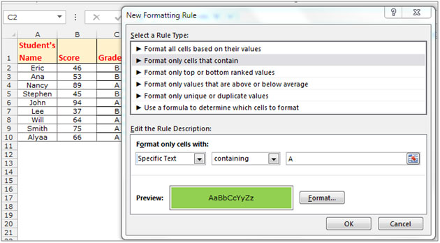
• Select the range C2:C10 by pressing the keys “CTRL+SHIFT+Down arrow key”.
• Go to the “Home Tab” in the “Styles” group and select “New Rule” from the “Conditional Formatting” drop down menu.
• The “New Formatting Rule” dialog box will appear.
• Select therule type “Format only cells that contain”. In the “Edit the Rule Description” dropdown select “Specific Text.
• In the 2nd drop menu select “Containing” and type “A” in the box.
• The “Format” option is showing in the belowdialog box. Click on the “Format” icon, then the “Format Cells” dialog box will appear. In the “Fill” tab select the green color and click on ok.
• The selected color will display in the “Preview” box and then click on ok.

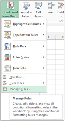
• Now select “Manage Rule” from the “Conditional Formatting” drop down menu.

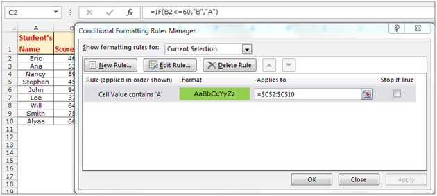
• The “Conditional Formatting Rules Manager” dialog box will appear..

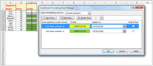
• Click on “New Rule” then again the “New Formatting Rule” dialog box will be activated.
• Select a rule type “Format only cells that contain”. In the “Edit the Rule Description” box select “Specific Text” from the drop down menu.
• In the 2nd drop down menu select “Containing” and type “B” in the box.
• The “Format” option is showing in the below dialog box. Click on “Format” icon, the “Format Cells” dialog box will appear. In the “Fill” tab select the yellow color and click on ok.
• In the “Conditional Formatting Rules Manager”dialog box click on apply then click on ok.

After using the Conditional Formatting conditions for all grades you will get the data as the below snapshot. Also if once you update the score the grade will be automatically updated.

If you liked our blogs, share it with your friends on Facebook. And also you can follow us on Twitter and Facebook.
We would love to hear from you, do let us know how we can improve, complement or innovate our work and make it better for you. Write us at info@exceltip.com