The SUMIF function is a useful function when it comes to summing up values based on some given condition. But there are times when you will face some difficulties working with the function. You will notice that the SUMIF function is not working properly or returning inaccurate results. This mostly happens when you are new t0 this function and haven't used it enough. It doesn't mean that it can't happen to experienced Excel players. Excel surprises us with its secrets.
There can be many reasons behind SUMIF's inaccuracy. In this article we will discuss all the cases in which SUMIF function may not work and how you can get it working.
Before we discuss issue points with SUMIF function in detail, check these in your formula. You may get your SUMIF formula working.
Now, if those haven't helped, you will get the SUMIF function working using below methods.
Syntactical error is pretty common mistake among the new users. Even Experienced users can make syntactical error while using the SUMIF function. So first let's see the syntax of SUMIF function.
Generic Excel SUMIF Formula:
You can learn all about SUMIF function here.
So the first argument is a range that contains your condition. The condition will be checked in this range only.
The second argument is condition itself. This is the condition that you want to check in the condition_range.
sum_range: The it is the range in that you want to some.
So we had a quick summery of the SUMIF function. Now let's see what syntactical mistakes you can do while using the SUMIF function.
Defining Criteria Mistakes
Most of the mistakes are done when we define criteria. It is due to the variation of data. The criteria in SUMIF is defined differently in different scenarios. To understand it, let's see some example.
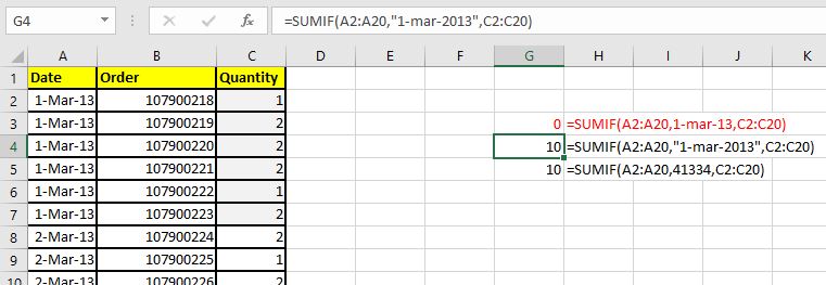
Here I have a data set.

Let's say I need to sum quantity of date 1-Mar-13.
So we write this formula.
| =SUMIF(A2:A20,1-mar-13,C2:C20) |
Will it work? Correct! this SUMIF formula will not work. It will return 0. Why?
The data we are working with is formatted as date. And dates in Excel are actually a numbers. And n number can be written without quotes as criteria. But still excel does not return the correct answer.
Actually, in SUMIF in excel, accepts date as text in criteria (if not formatted as serial number). So if you write this formula, it will return the correct answer.
| =SUMIF(A2:A20,"1-mar-13",C2:C20) |
ort
| =SUMIF(A2:A20,"1-mar-2013",C2:C20) |
The number equivalent of 1-mar-13 is 41334. So if I write this formula, it will return the correct answer.
| =SUMIF(A2:A20,41334,C2:C20) |
Note that I didn't use any quotes in this case. When we give number criteria, we don't need to use quotes.

So this one was the one case. You need to specially careful when you work with dates. They get messy very easily. So if your formula includes dates in it, check if it is in right format. Sometimes when we import data from other sources, dates aren't imported in accepted formats. So first check and correct the dates before using them.
Mistakes While Using Comparison Operator in SUMIF Function
Let's take another example. This time let's sum up the quantity of dates later than 1-Mar-13. For this the correct syntax is"
| =SUMIF(A2:A20,">1-Mar-13",C2:C20) |
Not this:
| =SUMIF(A2:A20,A2:A20>"1-Mar-13",C2:C20) |
We don't include the criteria range in criteria because we already told SUMIF the range in which to look.
Now if the criteria is in some cell, let's say in F3, than how would you use SUMIF function. Will the below formula work?
| =SUMIF(A2:A20,">F3",C2:C20) |
NO.
Will this.
| =SUMIF(A2:A20,>F3,C2:C20) |
NO.
This one should do than:
| =SUMIF(A2:A20,>"F3",C2:C20) |
A big NO. When we use comparison operators, we use ampersand to between operator and the range. The operator should be enclosed in quotes.
The SUMIF formula will work properly.
| =SUMIF(A2:A20,">"&F3,C2:C20) |

Note: When you need to sum values if a value matches exactly in criteria range, you don't need to use equal to sign "=". You just write that value or give the reference of that value at place of criteria, as we did in the first example.
I have noticed that some new users use the below syntax when they want an exact match.
| =SUMIF(A2:A20,A2:A20=F3,C2:C20) |
This too much wrong. This SUMIF will not work. When using reference as criteria for exact matches you just need to mention the reference. The below formula will sum all quantities of date written in cell F3:
| =SUMIF(A2:A20,F3,C2:C20) |
So these are some syntactical mistakes that can be the reason behind SUMIF not working. Let's see some other reasons.
A little bit of this, we have discussed in the previous section. But there is more to it.
The SUMIF function deals with numbers. Of course only numbers can be summed up. So first you need to check the sum range, if it is in the proper number format.
When we import data from other sources, it is common to have irregular data formats. It is very likely to have numbers formatted as text. In that case the numbers will not summed up. See the below example.

You can see that sum range contains text values instead of numbers. And since text values can't be summed up, the result we get is 0. The green corner in the cell indicates the the numbers are formatted as text.
It is possible that your range contains mixed formats. It is possible that only few numbers are formatted as text and rest are numbers. In that case those text formatted numbers will not be summed up and you will get an inaccurate result.
How to solve this
To fix this problem, select one cell that contains numbers and text and CTRL+SPACE to select entire column. Now click on the little exclamation mark on the left of the cell. Here you will see an option of "Convert to numbers" on second place. Click on it and you will have all the numbers in selected range converted to number format.

This is one solution. But if you are not able to do this. Use the VALUE function to convert text into numbers. The VALUE function coverts any formatted number into number format (even dates and times).
So this how it works. Use a column to convert all the numbers into values using the VALUE function and then value paste it. And then use that in the formula.

Date and Time Formatted Value Summation with SUMIF.
SUMIF may not visibly work when you try to sum up times. Yes visibly. See the below example.
Here I have time in HH:MM:SS format. And I want to sum up the hours of date 1-mar-13. So I use the formula:
| =SUMIF(A2:A20,F3,C2:C20) |
The formula is absolutely correct but the answer I am getting is not looking right.

Why am I getting 0.5. Shouldn't it return 12:00:00. Is it incorrect? No. The answer is write. As I said earlier, in Excel the time and date is treated differently. In Excel, 1 hour is equal to 1/24 unit. (I recommend you to understand excel date and time logic in detail. You can learn it here) So 12 hour will be equal to 0.5.
If you want to see the result in hours convert the cell format of G3 to time format.
Right click on the cell and click on the format cell. Here select the time format. And it is done. You can see that the result is converted to the correct format and returns an understandable result.

If for any reason, the SUMIF function is not working, no matter what you do, use an alternative formula. Here this formula uses SUMPRODUCT function.
For example if you want to do the same thing as above, we can use the SUMPRODUCT function to do so:
We want to sum range D2:D20 if date is equal to F3. So write this formula.
| =SUMPRODUCT(D2:D20,--(A2:A20=F3)) |
The order of the variables doesn't matter. The below formula will work perfectly fine:
| =SUMPRODUCT(--(A2:A20=F3),D2:D20) |
or this,
| =SUMPRODUCT(--(F3=A2:A20),D2:D20) |
You can learn about summing up with condition using SUMPRODUCT function here. The SUMPRODUCT function is very flexible and versatile function. I recommend you to understand it thoroughly.
So yeah guys, this is how you can solve the issue if SUMIF function isn't working. I have covered every possible reason that can cause SUMIF's unusual behavior. I hope it helped you. If it didn't, let me know it in the comments section below. If you have some new insight, share that too in the comments section below.
Related Articles:
13 Methods of How to Speed Up Excel | Excel is fast enough to calculate 6.6 million formulas in 1 second in Ideal conditions with normal configuration PC. But sometimes we observe excel files doing calculation slower than snails. There are many reasons behind this slower performance. If we can Identify them, we can make our formulas calculate faster.
Center Excel Sheet Horizontally and Vertically on Excel Page : Microsoft Excel allows you to align worksheet on a page, you can change margins, specify custom margins, or center the worksheet horizontally or vertically on the page. Page margins are the blank spaces between the worksheet data and the edges of the printed page
Split a Cell Diagonally in Microsoft Excel 2016 : To split cells diagonally we use the cell formatting and insert a diagonally dividing line into the cell. This separates the cells diagonally visually.
How do I Insert a Check Mark in Excel 2016 : To insert a checkmark in Excel Cell we use the symbols in Excel. Set the fonts to wingdings and use the formula Char(252) to get the symbol of a check mark.
How to disable Scroll Lock in Excel : Arrow keys in excel move your cell up, down, Left & Right. But this feature is only applicable when Scroll Lock in Excel is disabled. Scroll Lock in Excel is used to scroll up, down, left & right your worksheet not the cell. So this article will help you how to check scroll lock status and how to disable it?
What to do If Excel Break Links Not Working : When we work with several excel files and use formula to get the work done, we intentionally or unintentionally create links between different files. Normal formula links can be easily broken by using break links option.
Popular Articles:
50 Excel Shortcuts to Increase Your Productivity | Get faster at your task. These 50 shortcuts will make you work even faster on Excel.
How to use Excel VLOOKUP Function| This is one of the most used and popular functions of excel that is used to lookup value from different ranges and sheets.
How to use the Excel COUNTIF Function| Count values with conditions using this amazing function. You don't need to filter your data to count specific value. Countif function is essential to prepare your dashboard.
How to Use SUMIF Function in Excel | This is another dashboard essential function. This helps you sum up values on specific conditions.
The applications/code on this site are distributed as is and without warranties or liability. In no event shall the owner of the copyrights, or the authors of the applications/code be liable for any loss of profit, any problems or any damage resulting from the use or evaluation of the applications/code.