The Transpose function is an array function which is used to rotate the contents of columns to rows and rows to columns in Microsoft Excel. Microsoft Excel has 2 options to use the Transpose Function.
Let’s take an example and understand how we can use the Transpose function.
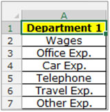
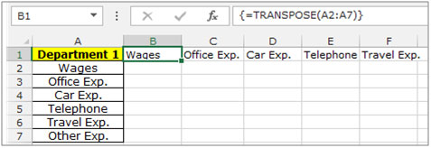
I have a table in range A2:A7 which contains the Expenses for a particular department. To transpose all the contents follow the below mentioned steps:-

Use the Transpose function with array

Use the Transpose feature in Excel

Below you can find more example to learn about Transpose:-
How to transpose cells in Microsoft Excel
How to transposing Values from Columns into Rows, and Vice Versa
How to Transpose in Microsoft Excel 2007
How to Copy Vertical and Paste Horizontal in Microsoft Excel
If you liked our blogs, share it with your friends on Facebook. And also you can follow us on Twitter and Facebook.
We would love to hear from you, do let us know how we can improve, complement or innovate our work and make it better for you. Write us at info@exceltip.com
The applications/code on this site are distributed as is and without warranties or liability. In no event shall the owner of the copyrights, or the authors of the applications/code be liable for any loss of profit, any problems or any damage resulting from the use or evaluation of the applications/code.
Suppose that........we have 10 phone numbers in a row. I want that it's all numbers in one cell....... With , sign
Create the reference going the direction of the existing data. Highlight references and bring up the find/replace dialog box (ctrl+F) and then replace = with D= or something similar.
Once that is done take the new reference, copy it, select where you want the data to be and paste special -> transpose.
Select the new data open find replace and replace D= with =.
All done
When I try to replace = with D=, I get the following error:
Excel cannot find any data to replace. Check if your search formatting and criteria are defined correctly.. .. it may be a protected sheet.
It's not protected I checked... I have no idea why this error is coming up.
Help is appreciated.
Thanks!
"If you like copy& paste transpose formula from one worksheet to another , first method works. Second method is better, but if you simply copy&paste special with transpose u have to include worksheet-name.
make this:
first: in worksheet with name 'source'
cell a1: value 2000
cell b1: value 2001
cell c1 :value 2002
cell a2: formula: '=source!A$1'
cell b2: formula: '=source!B$1'
cell c2: formula: '=source!C$1'
now select range A2:C2
Copy
select a5
past special formula transpose
done! "
"make this:
first:
cell a1: value 2000
cell b1: value 2001
cell c1 :value 2002
cell a2: formula: '=A$1'
cell b2: formula: '=B$1'
cell c2: formula: '=C$1'
now select range A2:C2
Copy
select a5
past special formula transpose
done!"