How to Divide an Amount into Equal Payments in Excel

As I have mentioned in many of my blogs that a SUMPRODUCT is a very versatile function and can be used for multiple purposes. In this article, we will see how we can use this function to count values with multiple or criterias.

Generic SUMPRODUCT Formula to Count With Multiple Or Criteria

Criteria1: This is any criteria that returns an array of TRUE and FALSE.

Criteria2: This is the next criteria that you want to check. Similarly you can have as many as criterias you want.

The above generic formula is modified often to suit the requirements to count with multiple OR criteria. But the base formula is this. First we will see how this works through an example and after that we will discuss other scenarios where you will need to modify this formula a little.

Problem:

The price in a cell should be divided accurately into 5 similar payments. When simply dividing the price $88.04 by 5 and rounding the result to two decimal places, we get individual payments of $17.61. However, this would add up to a total payment of $88.05, which is not the exact amount we begin with. Therefore, we want to calculate 5 similar numbers that add up to the total amount.

Solution:

First Calculate the first payment by dividing the price by 5 and rounding the result.

Use the ROUND function in the following formula:

=ROUND(B1/5,2)

Step 2:

Calculate each remaining payment.

Use the ROUND, SUM, and ROW functions in the following formula:

=ROUND(($B$1-SUM($B$2:B2))/(5-ROW()+ROW($B$2)),2)

Example:

Count Users If Dealer Code Matches Or Year Using SUMPRODUCT

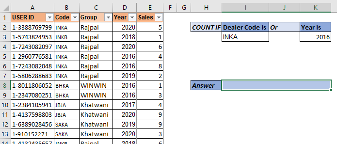
So here we have a data set of salespeople. The data contains many columns. What we need to do is to count the number of users who have code "INKA" or year is "2016". Make sure that if someone has both (code as "inka" and year 2016) should be counted as 1.

So, hear we have two criteria. We use the above mentioned SUMPRODUCT formula:

Here, code and year are named ranges. This returns 7. 

In the data we have  5 records of INKA code and 4 records of year 2016. But 2 records have both "INKA" and 2016 as code and year respectively. And these records are counted as 1. And this is how we get 7.

Let's see how it works?

So let's have a look at how the formula is solved step by step, then I will discuss how it works.

• • =SUMPRODUCT(--(((Code=I3)+(Year=K3))>0))
  • SUMPRODUCT(--(({TRUE;FALSE;TRUE;TRUE;TRUE;TRUE;...}+{FALSE;FALSE;FALSE;TRUE;TRUE;...})>0))
  • SUMPRODUCT(--(({1;0;1;2;2;1;1;1;0;0;0;0;0;0;0;0;0;0;0;0})>0))
  • SUMPRODUCT(--({TRUE;FALSE;TRUE;TRUE;TRUE;TRUE;TRUE;...})
  • SUMPRODUCT({1;0;1;1;1;1;1;1;0;0;0;0;0;0;0;0;0;0;0;0})

7

The double negative (--) signs are used to convert boolean values into 1s and 0s. So each TRUE value in the array is converted into 1 and FALSE into 0. 

Adding More Or Criterias To Count Using SUMPRODUCT, So if you need to add more or criterias to count, you can just add criteria using + sign to the function. 

For example, if you want to add another criteria to the above formula so that it adds the number of employees who have sold more than 5 products. The SUMPRODUCT formula will simply look like this:

Simple! isn't it?

But let's say you want to have two criterias from Code range. Let's say you want to count "INKB". Then how do you do this? One method is using the above technique but that would be repetitive. Let's say I want to add 10 more criterias from the same range. In such cases this technique is not that smart for counting with SUMPRODUCT.

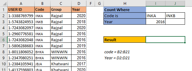
Let's say we have data arranged like this.

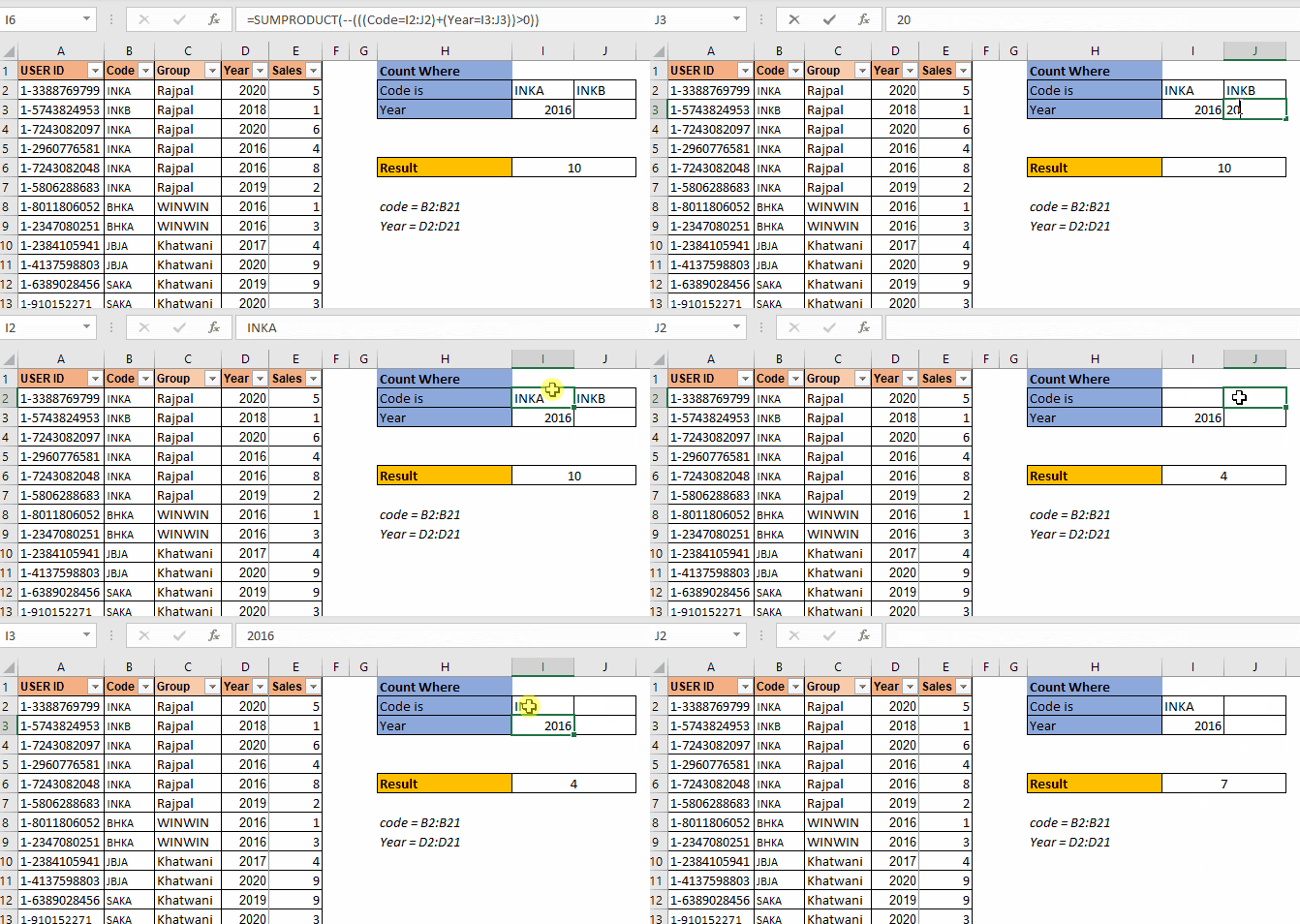
The criteria codes are in one row I2:J2. The arrangement of data is important here. The SUMPRODUCT formula for 3 OR criteria count setting will be:

This is the SUMPRODUCT formula to count with multiple criteria when multiple criteria from one range is written in row.

The above formula returns the correct answer which is 10. 

If you type any year in J3, the formula will add that count too.

This is used when the criterias are in one row. Will it work when the criterias in one column for the same range? No. It won't.

In this example we have multiple codes to count but these type codes are written in one column. When we use the above SUMPRODUCT formula, we get ans #N/A error. We will not get into how this error comes as this makes this article too long. Let's see how we can make this work.

To make this formula work, you need to wrap the code criteria in TRANSPOSE function. This will get the formula working.

This is the formula for counting with multiple or conditions in the same range when criteria is listed in a column.

Here are all the observational notes regarding using the formula. 

Notes:

1. The formula works for text and numbers both.
2. The lookup values can be given as cell reference or directly using quote symbol ( " ) in the formula as arguments.

Hope you understood How to Divide an Amount into Equal Payments While Avoiding Division / Rounding Errors in Excel. Explore more articles on Excel lookup value & Excel 2019 functions here. If you liked our blogs, share it with your friends on Facebook. And also you can follow us on Twitter and Facebook. We would love to hear from you, do let us know how we can improve, complement or innovate our work and make it better for you. Write to us at info@exceltip.com.

Related Articles

Use INDEX and MATCH to Lookup Value : INDEX & MATCH function to look up value as required.

SUM range with INDEX in Excel : Use INDEX function to find the SUM of the values as required.

How to use the INDEX function in Excel : Find the INDEX of an array using the INDEX function explained with an example.

How to use the MATCH function in Excel : Find the MATCH in the array using the INDEX value inside MATCH function explained with example.

How to use LOOKUP function in Excel : Find the lookup value in the array using the LOOKUP function explained with an example.

Popular Articles :

How to use the IF Function in Excel : The IF statement in Excel checks the condition and returns a specific value if the condition is TRUE or returns another specific value if FALSE.

How to use the VLOOKUP Function in Excel : This is one of the most used and popular functions of excel that is used to lookup value from different ranges and sheets. 

How to Use SUMIF Function in Excel : This is another dashboard essential function. This helps you sum up values on specific conditions.

How to use the COUNTIF Function in Excel : Count values with conditions using this amazing function. You don't need to filter your data to count specific values. Countif function is essential to prepare your dashboard.