Format Cells Contains Formula in Microsoft Excel

In this article we will learn how to format the cells which is containing the formulas in Microsoft Excel.

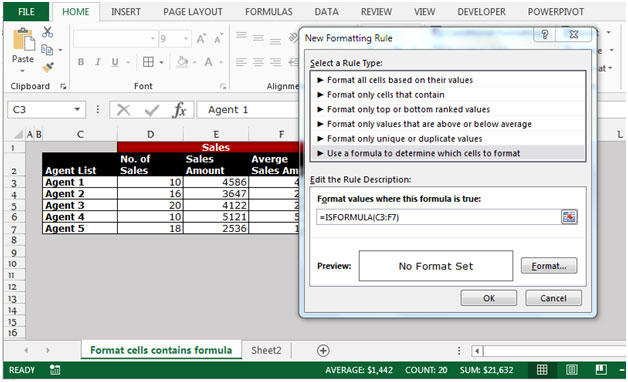
To format the cells which contain formulas, we use the Conditional Formatting feature along with the ISFORMULA function in Microsoft Excel.

Conditional Formatting: -Conditional Formatting is used to highlight the important points with color in a report based on certain conditions.

ISFORMULA-This function is used to check whether a cell reference contains a formula and it returns a True or False.

For Example - We have this Excel data as shown below -

We need to check whether cell E3 containsa formula or not.

To check, follow the below given steps:-

Select the cell F3 and write the formula.
=ISFORMULA(E3), press Enter on the keyboard.
The function will return true.
It means cell E3 contains a formula.

Let’s take an example to understand how we can highlight the cells which contain formulas.

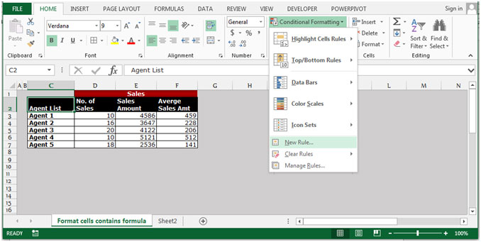
We have data in range C2:G7, in which column C contains Agents name, column D contains No. of sales, column E contains sales amount and column F contains Average sales amount. We need to highlight the cells which contain the formula.

Follow the below given steps:-

Select the data range C3:F7.
Go to the Home Tab.
Select Conditional Formatting from the Styles group.
From the Conditional formatting drop down menu, select New Rule.

The New Formatting Rule dialog box will appear.
Click on “Use a formula to determine which cells to format” from Select a Rule type.
Write the formula in Formula tab.
=ISFORMULA(C3:F7)

Click on Format button.
The Format Cells dialog box will appear.
In the Fill tab, choose the color as per the requirement.
Click on OK on the New Formatting Rule dialog box.

Click on OK on the Format Cells dialog box.

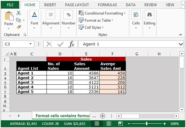
All cells which contain formulas will get highlighted with the chosen color. This is the way we can highlight the cells containing formulas in an Excel sheet by using the Conditional Formatting option along with the ISFORMULA function.

If you liked our blogs, share it with your friends on Facebook. And also you can follow us on Twitter and Facebook.
We would love to hear from you, do let us know how we can improve, complement or innovate our work and make it better for you. Write us at info@exceltip.com

Chad T. Lower
December 4, 2014 at 10:57 pm

Are you meaning to refer to 2013? I can't find this functionality in 2010 (although wish I could).

Reply ↓