How to Highlight Duplicates in Multiple Ranges in Excel

When you want to know what values are shared in 2 or more columns, highlighting the duplicate values is the best way to see them visually.

In this article, we will learn how to highlight duplicate values in two or more columns
Highlight Duplicate in Two or More Ranges
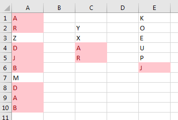
Here, I want you to highlight duplicate in ranges A1:A10, C2:C5 and D1:D6. Follow these steps:
1. To highlight duplicates, select all ranges. To select non-adjacent ranges, hold the CTRL key and use the mouse to select ranges.

2. Now go to Home->Conditional Formatting->Highlight Cells Rules->Duplicate Values.

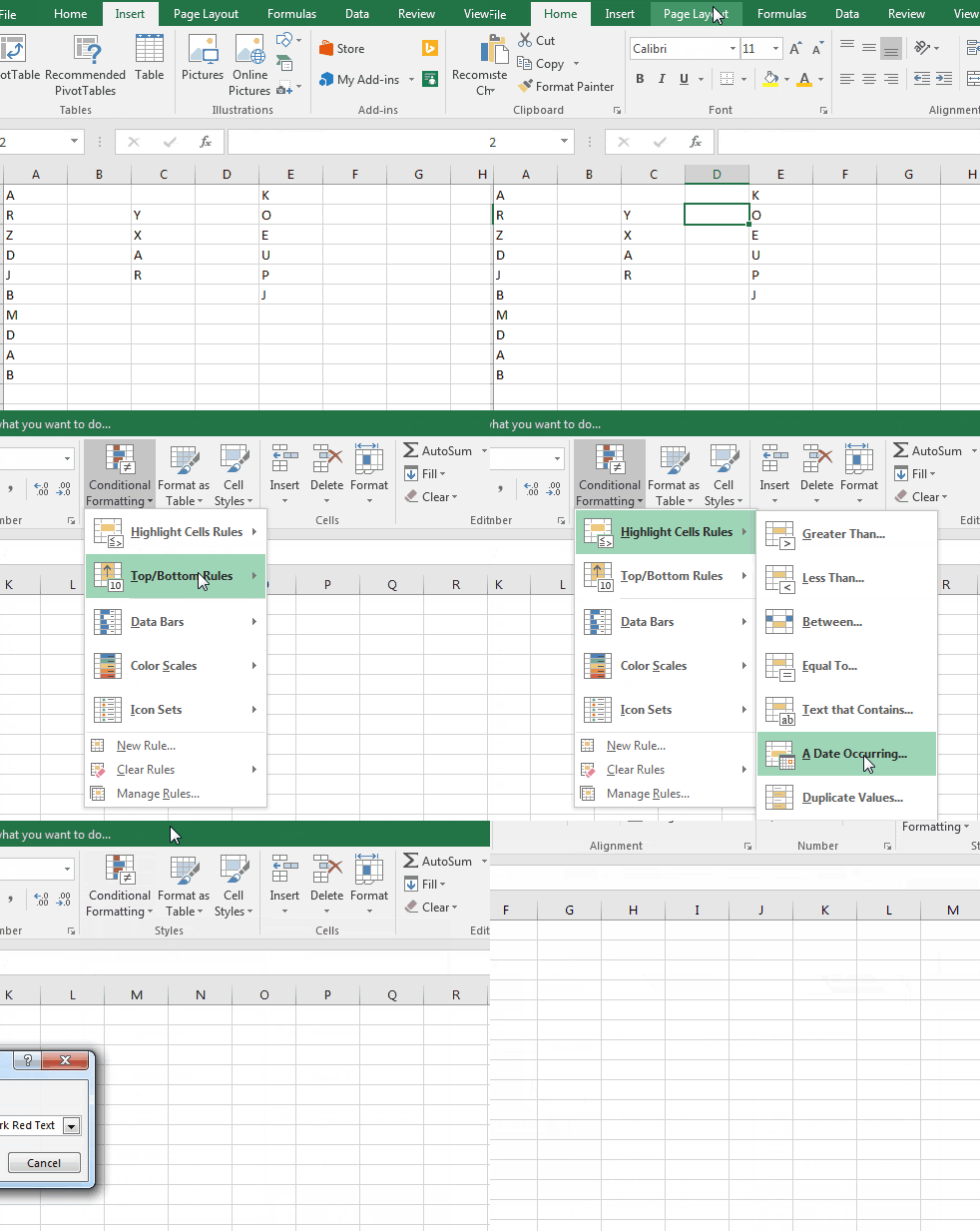
(Or you can use ALT>H>L>H>D>ENTER sequential shortcut to highlight duplicates)
3. Hit Enter or click OK. (before you hit enter, you can see in a small drop-down, an option is available to highlight duplicates or unique values. And the default formatting option. You may select whatever you like.
You can see each duplicate value highlighted by colour.
Alternate method:

How to find duplicate in Excel by using Conditional Formatting?

Let’s take another example to understand how we can find duplicates.

We have data in range A1:C15. Column A contains Student name, column B contains Mobile no. and column c contains Email Id.
Now, we want to find out the duplicates.

Select the range A2:C15.
Go to the “Home Tab” and then in the “Styles” group, select “New Rule” from the Conditional Formatting dropdown menu.

“New Formatting Rule” dialog box will appear. Now, select a rule type “Use a formula to determine which cells to format”.

Write the formula in the box of “Format values where this formula is true:”
=COUNTIF($A$2:$C$15,A1)=2
Click on “Format” button. A ‘Format Cells’ dialog box will appear.
Go to Fill tab and Font, choose the color as per the requirement and click on OK.

All duplicates will get highlighted with the color.

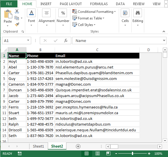
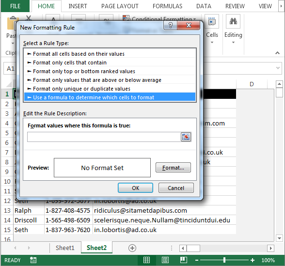
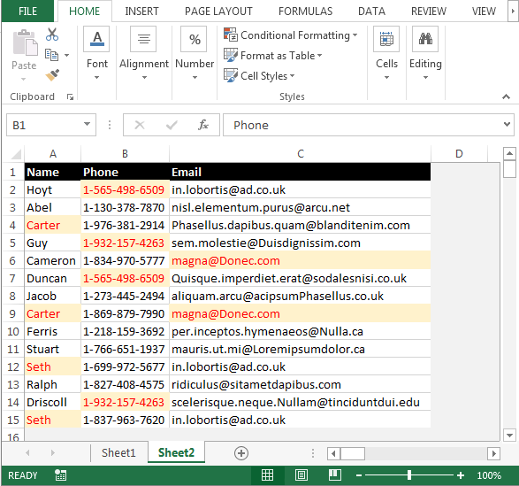
This is how we can find duplicates in Microsoft Excel.

Download - Highlight Duplicates in Excel - xlsx
It is damn easy to highlight duplicate values in excel. Isn’t it? But if you have any questions regarding this topic or any other topic, feel free to ask it in the comments section below. I would love to interact with excel users like you.