How to Retrieve a value from a reference grid according to index values Save in Excel

In this article, we will learn How to Retrieve a value from a reference grid according to index values Save in Excel

Scenario :

Many times when working with long unscattered data, we need to first clean data before working on it. It takes time and you just wanted to extract some queries. To extract data, you generally use the VLOOKUP function. But when we have long data with many column fields, then it gets messy because VLOOKUP function requires the correct column index as number, or else the formula returns error. Right there, below is the formula explanation for this kind of problem.

How to Solve the Problem?

For the formula to understand first we need to revise a little about the following functions

1. INDEX function
2. MATCH function

Now we will make a formula using the above functions. Match function will return the index of the lookup value1 in the row header field. And another MATCH function will return the index of the lookup value 2 in the column header field. The index numbers will now be fed into the INDEX function to get the values under the lookup value from the table data.

Generic Formula:

data : array of values inside the table without headers

lookup_value1 : value to lookup in the row_header.

row_headers : Row Index array to lookup.

lookup_value1 : value to lookup in the column_header.

column_headers : column Index array to lookup.

Example :

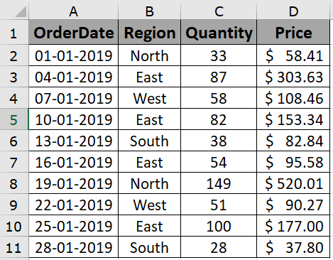
All of these might be confusing to understand. Let's understand how to use the function using an example. Here we have some sample order data and we need to find the missing data related to the given value in the table.

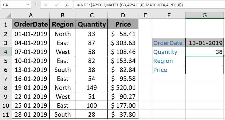
Here we need to find the order details like Quantity, region and price for the order placed on 13-01-2019.

Use the formula:

Explanation:

1. MATCH function returns the index of the matched value in the given 1D array (horizontal or vertical).
2. MATCH(F4,A1:D1,0) returns 3 as index.
3. MATCH(G3,A2:A11,0) returns 5 as Index
4. INDEX function will return the 5th element (starting from 2nd Row) in the 3rd column.

As you can see the quantity related to order placed on 13-01-2019 comes out to be 38. Now we can find the region from which the order was placed using the formula.

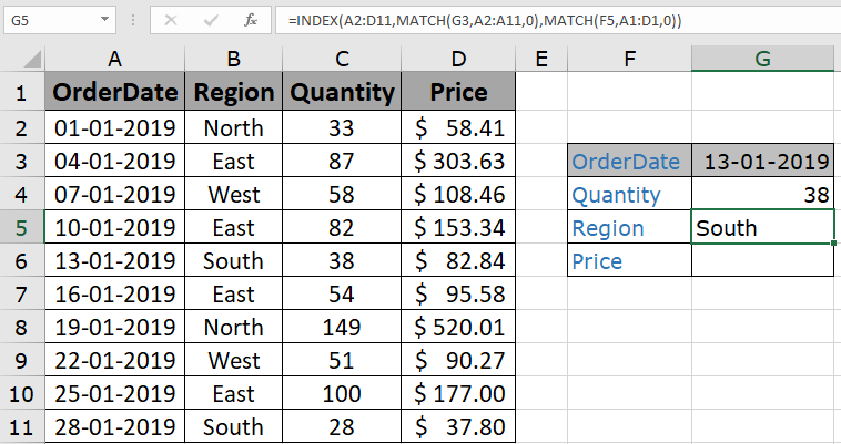
Use the formula:

As you can see the order was placed from the South region. Now get the price related to the order placed

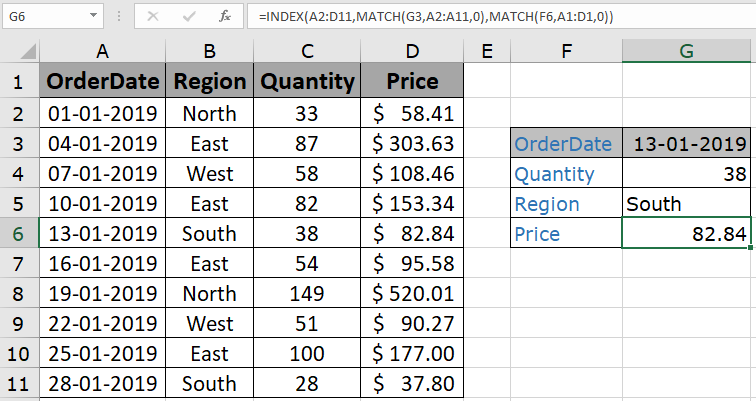
Use the formula:

As you can see price comes out to be 82.84. You noticed we extracted all details using one formula. The INDEX and MATCH combo is best to find one value from the table.

Here are all the observational notes regarding using the formula.

Notes:

1. The formula works for text and numbers both.
2. The function returns the #NA error if the lookup array argument to the MATCH function is not of the same length of the table array.
3. The formula returns an error if lookup_value doesn't match the value in the table lookup_array.
4. The function matches the exact value as the match type argument to the MATCH function is 0.
5. Use the argument -1 for less than, 0 for exact match and 1 for the greater than the lookup match.
6. The lookup values can be given as cell reference or directly using quote symbol ( " ) in the formula as arguments.

Hope you understood How to Retrieve a value from a reference grid according to index values Save in Excel. Explore more articles on Excel lookup value & Excel 2019 functions here. If you liked our blogs, share it with your friends on Facebook. And also you can follow us on Twitter and Facebook. We would love to hear from you, do let us know how we can improve, complement or innovate our work and make it better for you. Write to us at info@exceltip.com.

Related Articles

Use INDEX and MATCH to Lookup Value : INDEX & MATCH function to look up value as required.

SUM range with INDEX in Excel : Use INDEX function to find the SUM of the values as required.

How to use the INDEX function in Excel : Find the INDEX of an array using the INDEX function explained with an example.

How to use the MATCH function in Excel : Find the MATCH in the array using the INDEX value inside MATCH function explained with example.

How to use LOOKUP function in Excel : Find the lookup value in the array using the LOOKUP function explained with example.

Popular Articles :

How to use the IF Function in Excel : The IF statement in Excel checks the condition and returns a specific value if the condition is TRUE or returns another specific value if FALSE.

How to use the VLOOKUP Function in Excel : This is one of the most used and popular functions of excel that is used to lookup value from different ranges and sheets.

How to Use SUMIF Function in Excel : This is another dashboard essential function. This helps you sum up values on specific conditions.

How to use the COUNTIF Function in Excel : Count values with conditions using this amazing function. You don't need to filter your data to count specific values. Countif function is essential to prepare your dashboard.