Selecting/Formatting Cells Containing Errors in Microsoft Excel 2010

In this article we will learn how to select the cells that contain only errors, we will use the "Go-To" option. And if we need to format the cells containing errors, we will use the conditional formatting option along with the "ISERROR" function in Microsoft Excel 2010.

"Go-To Special": - This option is used to quickly re-direct to different cells in Excel.

Shortcut: F5 and Ctrl+G

Command button: Home tab> Select Find & Select >Select Go to Special

Conditional Formatting:-Conditional Formatting is used to highlight the important points with color in a report based on certain conditions.

ISERROR function- This function is used to check whether a value results in an error (#N/A, #VALUE!, #REF!, #DIV/0!, #NUM!, #NAME?, OR #NULL!) and it returns True or False.

The Syntax of “ISERROR” function: =ISERROR(Value)

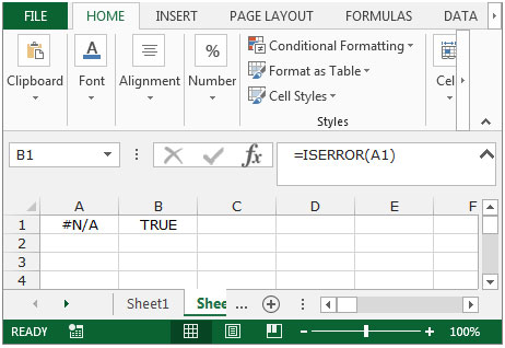
Let’s take an example to understand how we can select and format the cells that contain an error.

We have a sales report in which some cells contain formulas and an error is present in one or more of these cells. We need to select the cell(s) which contain the errors.

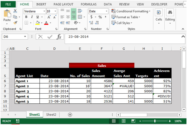
To select the cells which contain errors, follow the below given steps:-

In the Home tab from the editing group, click on Find & Select and select GoTo Special or you can press the shortcut key F5.

When we press the F5 key, the Go To dialog box will appear.
Click on the Special button in the bottom left corner.

The Go To Special dialog box will open.
Click on the Formulas option.
All formulas related options will get activated. Uncheck all the options except Errors.
Click on OK.

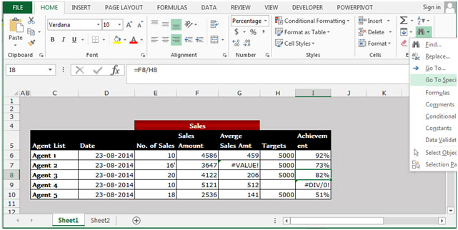
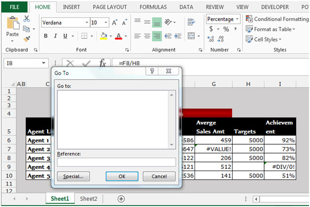
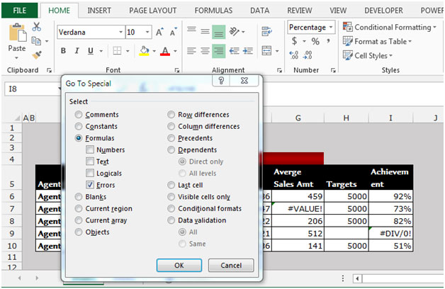
All the cells containing any type of error will get selected in the worksheet.

Thus, we can identify which cells contain the errors using this method.

To highlight the cells containing errors, follow the below given steps:-

Select the data range C6:I10.
Go to the Home Tab.
Select Conditional Formatting from the Styles group.
From the Conditional formatting drop down menu select New Rule.

The New Formatting Rule dialog box will appear.
Click on “Use a formula to determine which cells to format” from Select a Rule type.
Write the formula in the formula box.
=ISERROR(C6:I10).

Click on the Format button.
The Format Cells dialog box will appear.
In the Fill tab, choose the color as per the requirement.
Click on OK on the Format Cells dialog box.

Click on ok on the New Formatting Rule’s dialog box.

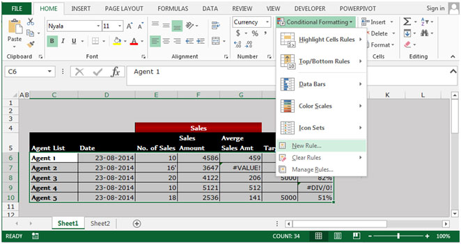
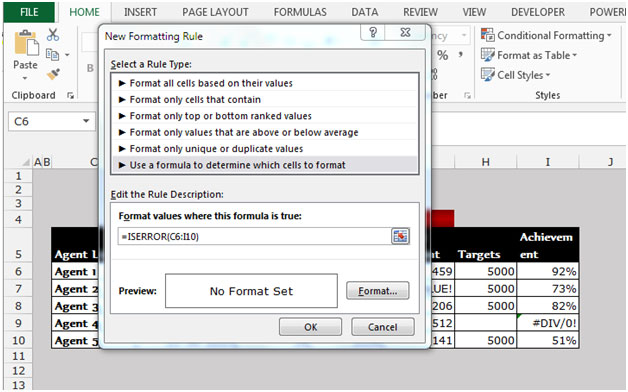
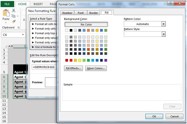
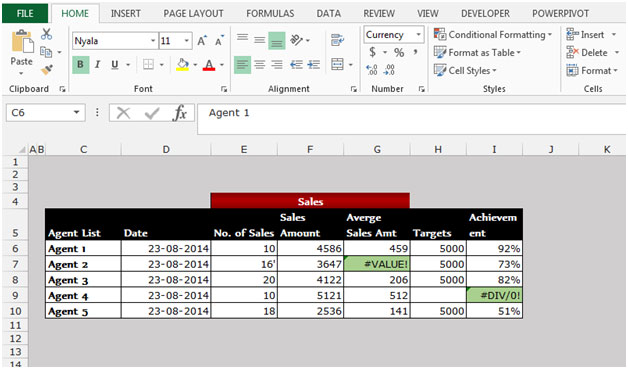
All the cells containing any type of error will be highlighted in the chosen color.

This is the way we can highlight the cells containing errors in an Excel sheet by using the Conditional Formatting option along with the ISERROR function.