Validating Data To Be Unique In Excel Range

What is Data Validation tool and how to use it to validate only unique values?

Data validation tool restricts the user to input data to ensure its accuracy and consistency in Excel. It guides the user to input the type of option which is necessary for your worksheet.

Here the problem is, we need to check if the cell has a value which is not repeated in the list it contains. If you want to learn more about Data validation in Excel, follow the link. Here we will just consider the problem, allow values only with no number.

How to solve the problem?

Here we have a task that allows entries which are unique in the list which means no repeated value is allowed. The use of functions and a tool will help us get through the problem.

1. Data validation tool
2. COUNTIF function

The formula be used in Data Validation tool. The formula checks the condition and returns True or False. Here the True means that the punctuation doesn't exist, so the tool accepts the value.

Generic formula:

Example :

All of these might be confusing to understand. So, let's test this formula via running it on the example shown below. Here we are preparing a product name list. But we don't any value to be repeated and whenever we enter a repeated value, it must show that this product Name is already there, try another Product name.

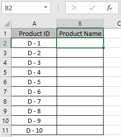
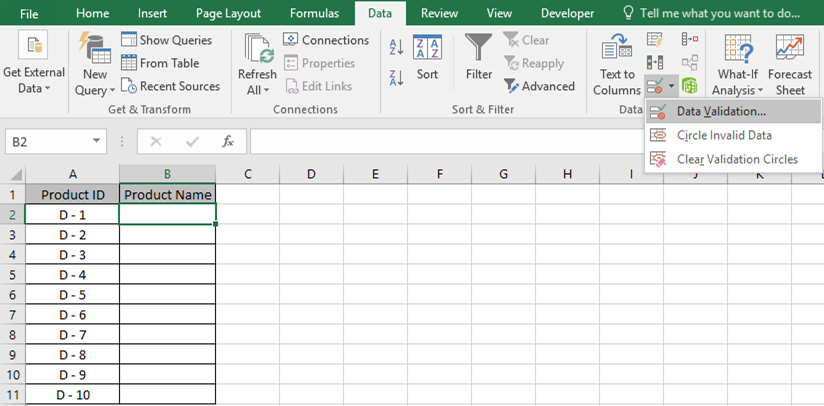
Select the cell B2, where the first Product name to be entered. Now Go to Data -> click Data Validation option -> Select Data Validation.

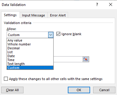
A Data Validation box appears in front with Settings. Under Allow list, select the Custom option from the drop down list.

Then the tool opens up the formula box. Here we will apply a data validation on the B2 cell to allow the user to input only unique values. Below is the formula to apply.

Use the formula:

Explanation

1. COUNTIF function counts the B2 value in the B column.
2. And returns the numerical count.
3. The <=1 checks if the count is less than or equals to 1, it returns TRUE and hence accepts the value. But if the count is more than 1, the formula returns FALSE and hence the value is rejected.

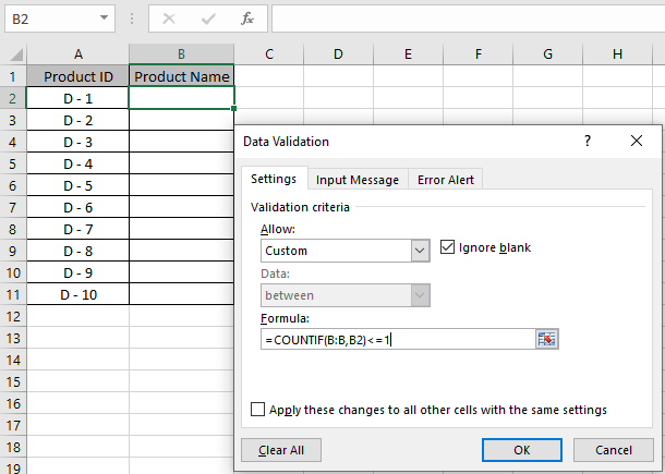
Click Ok to apply these changes. Now only B1 cell has the Data validation code, not the rest of the cell. So use our basic method of extending the formula to all the remaining cells. Use Ctrl + D till the cell you require to use the formula. Here the formula is extended to B11 cell.

Now your code is ready. As we entered the first product name it accepted. So we try the same value in further cell.

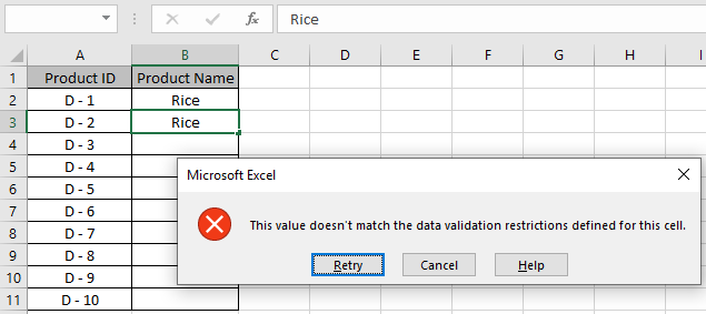
It throws an error "This value doesn't match the data validation restrictions defined for this cell". You can also customize the error message and alert message to let users know what values are prohibited. Edit alert and message as shown below.

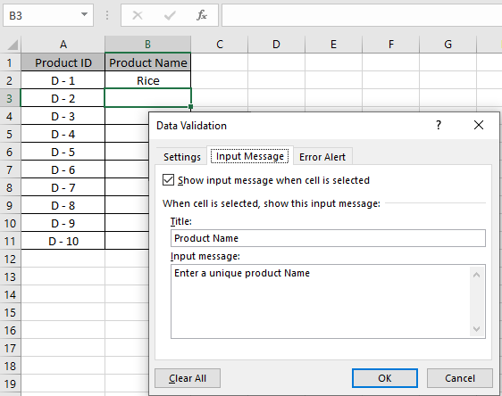
Input Alert message be typed in Input Message tab as shown in above image.

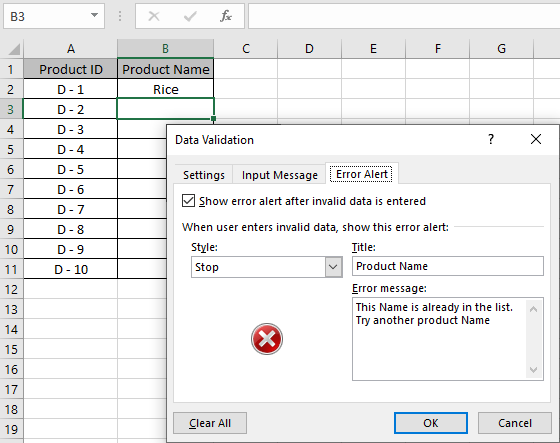
An Error Alert message be used in the Error Alert tab. Now click OK to get these changes.

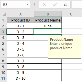
As you can see the Caution alert in the yellow box hanging below C2 cell. Now you can copy the Data validation format to the rest of the required cell using Ctrl + D.

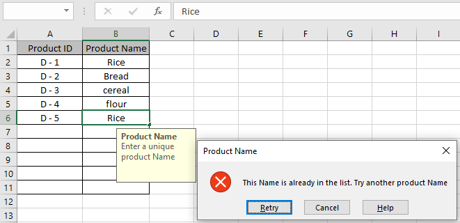
As you can see, now these cells will only accept unique values. You can apply the formula for the related column. The formula considers Rice, RICE, rice as the same values. So it rejects, if repeated.

Here are all the observational notes regarding using the formula.

Notes:

1. Apply the data validation tool to restrict the user to input invalid value, which doesn't satisfy the condition.
2. Data validation tool can work with numbers and text both.

Hope this article about How to validate only numbers in cells in Excel is explanatory. Find more articles on data validation tools with formulas here. If you liked our blogs, share it with your friends on Facebook. And also you can follow us on Twitter and Facebook. We would love to hear from you, do let us know how we can improve, complement or innovate our work and make it better for you. Write us at info@exceltip.com

Related Articles:

Data Validation in Excel : Restricts users to input value manually using this tool in Excel.

Way to use Vlookup function in Data Validation : allow values from the vlookup table in Excel.

Restrict Dates using Data Validation : allow dates in the cell which lays within Excel date format in Excel.

How to give the error messages in Data Validation : customize your data validation cell with error messages in Excel.

Create Drop Down Lists in Excel using Data Validation : restricts users to input data manually in Excel.

Popular Articles :

How to use the IF Function in Excel : The IF statement in Excel checks the condition and returns a specific value if the condition is TRUE or returns another specific value if FALSE.

How to use the VLOOKUP Function in Excel : This is one of the most used and popular functions of excel that is used to lookup value from different ranges and sheets.

How to use the SUMIF Function in Excel : This is another dashboard essential function. This helps you sum up values on specific conditions.

How to use the COUNTIF Function in Excel : Count values with conditions using this amazing function. You don't need to filter your data to count specific values. Countif function is essential to prepare your dashboard.